Dive into Deep Learning笔记——上

---

---

最后更新，2022.10.28
学习来自b站李沐课程Dive into Deep Learning，查漏补缺
文章内容并非全部来自于课程，还有自己的理解和加的其他东西

---

---

学到：
py3.8 jupyter torch相关 标量向量矩阵的运算求导 框架计算图自动求导 模型的底层实现过程
线性回归 softmax图像分类 多层感知机 正则 dropout Xavier初始化 自定义模型函数 NAS automl
卷积 LeNet AlexNet VGGNet NiN googleNet BN ResNet DenseNet GPU训练 图像增广 迁移学习
锚框 RCNN SSD YOLO centernet FCN 风格迁移…

---

S

1、
pd.get_dummies()特征提取，对文本特征做了onehot编码插入，其他不变

2、
如果训练数据过大，训练会发生梯度爆炸，可以把数据用log降下来，再z-score归一化

3、
训练和验证 预测 未来产生的数据集很有可能并不来自同一个分布（比如南方北方的区别、每年不同的气候变化、政策移民突然变多，比如模型训练发现训练集里贷款申请人的鞋子衣服与违约风险相关这种错误的关联，比如要图像分类的目标占据图片的大小被模型关注-有占1/4的有充满整个图像的），世界是一直变化的，解决办法用集成学习、不要太对训练数据过拟合、或对数据做统计分析处理 去掉不想让模型关注到的一些特征 加入环境变化特征 增加鲁棒性

4、
自定义模型函数，nn.Module的子类，只需要继承然后定义__init__(模型每层)和forward(计算输出) 反向自动求导不需要定义

5、
模型参数保存和读取

class MLP(nn.Module):
    ...
net = MLP()
torch.save(net.state_dict(), 'mlp.params')  # 保存模型参数到文件

clone = MLP() # 声明模型的构造
clone.load_state_dict(torch.load('mlp.params')) # 加载参数到模型中
clone.eval()
# 然后clone和net就一致了

6、
复杂模型中的很多超参数其实就是调出来的，一般都是调出多个不同参数的模型一起训练取最优，模型内部每一层机器是怎么学的、学到什么其实难以控制，并且不可解释性强
所以，不要太关注它有些层为什么是那样大小、通道数为什么是那个具体值，重要的是搞懂模型构造思想，以及参数设置不要偏离太多

7、
torchvision.transforms里有很多图像变换的东西，用于cv领域的数据增强
https://blog.csdn.net/qq_44766883/article/details/111320456

8、
如果数据集里正例样本很少的话（比如台风预测、欺诈预测），救需要对正样本做重采样、数据增强等方法，从数据上保证模型可以训练到很有用

9、
SGD优化算法调参影响大，有可能很好也会很差，Adam就比较稳定 也不需要怎么调参，适合不需要特别精确也不想更多调参的人用，SGD可能20分可能90分，Adam稳定70分

10、
图片归一化，对RGB图片是固定的参数-是大部分人实践出来的共识
rgb_mean = torch.tensor([0.485, 0.456, 0.406])
rgb_std = torch.tensor([0.229, 0.224, 0.225])
torchvision.transforms.Normalize(mean=rgb_mean, std=rgb_std)

线性回归

import torch

# # 参数初始化，第二个true代表需要更新，实际工作不会手动实现*
# w = torch.normal(0, 0.01, size=(2,1), requires_grad=True)
# b = torch.zeros(1, requires_grad=True)
# b.backward() # 反向传播
# print(b.grad)  # 梯度

def synthetic_data(w, b, num_examples):
    """生成y=Xw+b+噪声"""
    X = torch.normal(0, 1, (num_examples, len(w)))  # 均值0方差1的数据
    y = torch.matmul(X, w) + b
    y += torch.normal(0, 0.01, y.shape)
    return X, y.reshape((-1, 1))

true_w = torch.tensor([2, -3.4])
true_b = 4.2
features, labels = synthetic_data(true_w, true_b, 100)  # 生成特定参数的训练集XY假数据
print(features,labels)


from torch.utils import data
def load_array(data_arrays, batch_size, is_train=True):  #@save
    """构造一个PyTorch数据迭代器"""
    dataset = data.TensorDataset(*data_arrays)  # torch的dataset类型
    return data.DataLoader(dataset, batch_size, shuffle=is_train)
    # 随机挑选批次数据出来，shuffle=训练是需要打乱的

batch_size = 10
data_iter = load_array((features, labels), batch_size)
# 构造Python迭代器，并使用next从迭代器中获取第一项
next(iter(data_iter))

net = torch.nn.Sequential(torch.nn.Linear(2, 1))  # 线性回归，2 1是输入输出维度
net[0].weight.data.normal_(0, 0.01)  # 初始化w
net[0].bias.data.fill_(0)  # 初始化b
loss=torch.nn.MSELoss()  # 均方误差
trainer = torch.optim.SGD(net.parameters(), lr=0.3) # net.par.是模型的超参数，SGD只需要指定学习率

# 训练
num_epochs = 3
for epoch in range(num_epochs):
    for X, y in data_iter:
        l = loss(net(X) ,y)
        trainer.zero_grad() # 在每次更新梯度前都要trainer.zero_grad()，否则梯度会累加
        l.backward()
        trainer.step()  # 更新模型参数
    l = loss(net(features), labels)
    print(f'epoch {epoch + 1}, loss {l:f}')  # epoch 1, loss 0.000205

w = net[0].weight.data
print('w的估计误差：', true_w - w.reshape(true_w.shape))  #  tensor([0.0008, 0.0036])
b = net[0].bias.data
print('b的估计误差：', true_b - b)  # tensor([0.0065])

softmax图像分类

import torch
import torchvision
from torchvision import transforms  # 有各种数据集
from matplotlib import pyplot as plt
from torch.utils import data

# 通过ToTensor实例将图像数据从PIL类型变换成32位浮点数格式，
# 并除以255使得所有像素的数值均在0到1之间
trans=transforms.ToTensor() # 图片转tensor
mnist_train = torchvision.datasets.FashionMNIST(
    root="../data", train=True, transform=trans, download=True)
mnist_test = torchvision.datasets.FashionMNIST(
    root="../data", train=False, transform=trans, download=True)

print(len(mnist_train), len(mnist_test)) # 60000 10000
print(mnist_train[0][0].shape)  # torch.Size([1, 28, 28])

# Fashion-MNIST中包含的10个类别，分别为t-shirt（T恤）、trouser（裤子）、pullover（套衫）、dress（连衣裙）、
# coat（外套）、sandal（凉鞋）、shirt（衬衫）、sneaker（运动鞋）、bag（包）和ankle boot（短靴）。
# 以下函数用于在数字标签索引及其文本名称之间进行转换
def get_fashion_mnist_labels(labels):
    text_labels = ['t-shirt', 'trouser', 'pullover', 'dress', 'coat',
                   'sandal', 'shirt', 'sneaker', 'bag', 'ankle boot']
    return [text_labels[int(i)] for i in labels]

def show_images(imgs, num_rows, num_cols, titles=None, scale=1.5):  #@save
    figsize = (num_cols * scale, num_rows * scale)
    _, axes = plt.subplots(num_rows, num_cols, figsize=figsize)
    axes = axes.flatten()
    for i, (ax, img) in enumerate(zip(axes, imgs)):
        if torch.is_tensor(img):  # 图片张量
            ax.imshow(img.numpy())
        else:  # PIL图片
            ax.imshow(img)
        ax.axes.get_xaxis().set_visible(False)
        ax.axes.get_yaxis().set_visible(False)
        if titles:
            ax.set_title(titles[i])
    plt.show()
    return axes

# X, y = next(iter(data.DataLoader(mnist_train, batch_size=18)))
# show_images(X.reshape(18, 28, 28), 2, 9, titles=get_fashion_mnist_labels(y))

# 读取批量数据
# batch_size = 256
def get_dataloader_workers():  #@save
    """使用4个进程来读取数据"""
    return 0
# train_iter = data.DataLoader(mnist_train, batch_size, shuffle=True,
#                              num_workers=get_dataloader_workers())


# 整合图像读取到一个方法
def load_data_fashion_mnist(batch_size, resize=None):
    """下载Fashion-MNIST数据集，然后将其加载到内存中"""
    trans = [transforms.ToTensor()]
    if resize:
        trans.insert(0, transforms.Resize(resize))
    trans = transforms.Compose(trans)
    mnist_train = torchvision.datasets.FashionMNIST(
        root="../data", train=True, transform=trans, download=True)
    mnist_test = torchvision.datasets.FashionMNIST(
        root="../data", train=False, transform=trans, download=True)
    return (data.DataLoader(mnist_train, batch_size, shuffle=True,
                            num_workers=get_dataloader_workers()),
            data.DataLoader(mnist_test, batch_size, shuffle=False,
                            num_workers=get_dataloader_workers()))

# # 读取数据
# train_iter, test_iter = load_data_fashion_mnist(32, resize=64)
# for X, y in train_iter:
#     print(X.shape, X.dtype, y.shape, y.dtype)
#     # torch.Size([32, 1, 64, 64]) torch.float32 torch.Size([32]) torch.int64
#     break

batch_size = 256
train_iter, test_iter = load_data_fashion_mnist(batch_size)
# PyTorch不会隐式地调整输入的形状。因此，
# 我们在线性层前定义了展平层（flatten），来调整网络输入的形状
net = torch.nn.Sequential(torch.nn.Flatten(), torch.nn.Linear(784, 10))
def init_weights(m):
    if type(m) == torch.nn.Linear:
        torch.nn.init.normal_(m.weight, std=0.01)
net.apply(init_weights)  # 每一层权重初始化
loss = torch.nn.CrossEntropyLoss()  # 交叉熵
trainer = torch.optim.SGD(net.parameters(), lr=0.1)  # SGD


class Accumulator:
    """在n个变量上累加"""
    def __init__(self, n):
        self.data = [0.0] * n
    def add(self, *args):
        self.data = [a + float(b) for a, b in zip(self.data, args)]
    def reset(self):
        self.data = [0.0] * len(self.data)
    def __getitem__(self, idx):
        return self.data[idx]

def accuracy(y_hat, y):
    """计算预测正确的数量"""
    if len(y_hat.shape) > 1 and y_hat.shape[1] > 1:
        y_hat = y_hat.argmax(axis=1)
    cmp = y_hat.type(y.dtype) == y
    return float(cmp.type(y.dtype).sum())

def evaluate_accuracy(net, data_iter):
    """计算在指定数据集上模型的精度"""
    if isinstance(net, torch.nn.Module):
        net.eval()  # 将模型设置为评估模式
    metric = Accumulator(2)  # 正确预测数、预测总数
    with torch.no_grad():
        for X, y in data_iter:
            metric.add(accuracy(net(X), y), y.numel())
    return metric[0] / metric[1]

def train_epoch_ch3(net, train_iter, loss, updater):  #@save
    """训练模型一个迭代周期"""
    # 将模型设置为训练模式
    if isinstance(net, torch.nn.Module):
        net.train()
    # 训练损失总和、训练准确度总和、样本数
    metric = Accumulator(3)
    for X, y in train_iter:
        # 计算梯度并更新参数
        y_hat = net(X)
        l = loss(y_hat, y)
        if isinstance(updater, torch.optim.Optimizer):
            # 使用PyTorch内置的优化器和损失函数
            updater.zero_grad()
            l.mean().backward()
            updater.step()
        else:
            # 使用定制的优化器和损失函数
            l.sum().backward()
            updater(X.shape[0])
        metric.add(float(l.sum()), accuracy(y_hat, y), y.numel())
    # 返回训练损失和训练精度
    return metric[0] / metric[2], metric[1] / metric[2]

def train_ch3(net, train_iter, test_iter, loss, num_epochs, updater):
    """训练模型"""
    for epoch in range(num_epochs):
        train_metrics = train_epoch_ch3(net, train_iter, loss, updater)
        test_acc = evaluate_accuracy(net, test_iter)
        print(train_metrics)  # 打印loss和acc，(0.00175, 0.84773)
    train_loss, train_acc = train_metrics
    assert train_loss < 0.5, train_loss
    assert train_acc <= 1 and train_acc > 0.7, train_acc
    assert test_acc <= 1 and test_acc > 0.7, test_acc

num_epochs = 10
train_ch3(net, train_iter, test_iter, loss, num_epochs, trainer)

def predict_ch3(net, test_iter, n=6):  # 预测，并画图
    for X, y in test_iter:
        break
    trues = get_fashion_mnist_labels(y)
    preds = get_fashion_mnist_labels(net(X).argmax(axis=1))
    titles = [true +'\n' + pred for true, pred in zip(trues, preds)]
    show_images(X[0:n].reshape((n, 28, 28)), 1, n, titles=titles[0:n])

predict_ch3(net, test_iter)

多层感知机MLP

感知机本质上是一个二分类的问题：输入大于0就输出1，否则输出0

多层感知机MLP（multi-layer pecerptron）其实就像多层softmax回归，多了隐藏层，多了非线性激活函数
多层感知机的结构和BP差不多，BP神经网络是用BP算法进行训练的多层感知器模型

感知机和SVM的区别：
感知机目标找到一个超平面将各样本尽可能分离正确（有无数个）；SVM目标找到一个超平面不仅将各样本尽可能分离正确，还要使各样本离超平面距离最远（只有一个），SVM的泛化能力更强

多层感知机的隐藏层就是逐渐压缩或者先扩充再压缩，从高维输入一步步提取特征到低维空间输出

import torch
import torchvision
from torchvision import transforms  # 有各种数据集
from matplotlib import pyplot as plt
from torch.utils import data

def load_data_fashion_mnist(batch_size, resize=None):
    """下载Fashion-MNIST数据集，然后将其加载到内存中"""
    trans = [transforms.ToTensor()]
    if resize:
        trans.insert(0, transforms.Resize(resize))
    trans = transforms.Compose(trans)
    mnist_train = torchvision.datasets.FashionMNIST(
        root="../data", train=True, transform=trans, download=True)
    mnist_test = torchvision.datasets.FashionMNIST(
        root="../data", train=False, transform=trans, download=True)
    return (data.DataLoader(mnist_train, batch_size, shuffle=True),
            data.DataLoader(mnist_test, batch_size, shuffle=False))

batch_size = 256
train_iter, test_iter = load_data_fashion_mnist(batch_size)

# 模型参数初始化
num_inputs, num_outputs, num_hiddens = 784, 10, 256   # 隐藏层256
W1 = torch.nn.Parameter(torch.randn(
    num_inputs, num_hiddens, requires_grad=True) * 0.01)
b1 = torch.nn.Parameter(torch.zeros(num_hiddens, requires_grad=True))
W2 = torch.nn.Parameter(torch.randn(
    num_hiddens, num_outputs, requires_grad=True) * 0.01)
b2 = torch.nn.Parameter(torch.zeros(num_outputs, requires_grad=True))
params = [W1, b1, W2, b2]

def relu(X):
    a = torch.zeros_like(X)
    return torch.max(X, a)
def net(X):
    X = X.reshape((-1, num_inputs))
    H = relu(X@W1 + b1)  # 这里“@”代表矩阵乘法
    return (H@W2 + b2)


class Accumulator:
    """在n个变量上累加"""
    def __init__(self, n):
        self.data = [0.0] * n
    def add(self, *args):
        self.data = [a + float(b) for a, b in zip(self.data, args)]
    def reset(self):
        self.data = [0.0] * len(self.data)
    def __getitem__(self, idx):
        return self.data[idx]

def accuracy(y_hat, y):
    """计算预测正确的数量"""
    if len(y_hat.shape) > 1 and y_hat.shape[1] > 1:
        y_hat = y_hat.argmax(axis=1)
    cmp = y_hat.type(y.dtype) == y
    return float(cmp.type(y.dtype).sum())

def evaluate_accuracy(net, data_iter):
    """计算在指定数据集上模型的精度"""
    if isinstance(net, torch.nn.Module):
        net.eval()  # 将模型设置为评估模式
    metric = Accumulator(2)  # 正确预测数、预测总数
    with torch.no_grad():
        for X, y in data_iter:
            metric.add(accuracy(net(X), y), y.numel())
    return metric[0] / metric[1]

def train_epoch_ch3(net, train_iter, loss, updater):
    """训练模型一个迭代周期"""
    # 将模型设置为训练模式
    if isinstance(net, torch.nn.Module):
        net.train()
    # 训练损失总和、训练准确度总和、样本数
    metric = Accumulator(3)
    for X, y in train_iter:
        # 计算梯度并更新参数
        y_hat = net(X)
        l = loss(y_hat, y)
        if isinstance(updater, torch.optim.Optimizer):
            # 使用PyTorch内置的优化器和损失函数
            updater.zero_grad()
            l.mean().backward()
            updater.step()
        else:
            # 使用定制的优化器和损失函数
            l.sum().backward()
            updater(X.shape[0])
        metric.add(float(l.sum()), accuracy(y_hat, y), y.numel())
    # 返回训练损失和训练精度
    return metric[0] / metric[2], metric[1] / metric[2]

def train_ch3(net, train_iter, test_iter, loss, num_epochs, updater):
    """训练模型"""
    for epoch in range(num_epochs):
        train_metrics = train_epoch_ch3(net, train_iter, loss, updater)
        test_acc = evaluate_accuracy(net, test_iter)
        print(train_metrics)  # 打印loss和acc，(0.00175, 0.84773)
    train_loss, train_acc = train_metrics
    assert train_loss < 0.5, train_loss
    assert train_acc <= 1 and train_acc > 0.7, train_acc
    assert test_acc <= 1 and test_acc > 0.7, test_acc

loss = torch.nn.CrossEntropyLoss(reduction='none')
num_epochs, lr = 3, 0.3
updater = torch.optim.SGD(params, lr=lr)
train_ch3(net, train_iter, test_iter, loss, num_epochs, updater)

def show_images(imgs, num_rows, num_cols, titles=None, scale=1.5):
    figsize = (num_cols * scale, num_rows * scale)
    _, axes = plt.subplots(num_rows, num_cols, figsize=figsize)
    axes = axes.flatten()
    for i, (ax, img) in enumerate(zip(axes, imgs)):
        if torch.is_tensor(img):  # 图片张量
            ax.imshow(img.numpy())
        else:  # PIL图片
            ax.imshow(img)
        ax.axes.get_xaxis().set_visible(False)
        ax.axes.get_yaxis().set_visible(False)
        if titles:
            ax.set_title(titles[i])
    plt.show()
    return axes
def get_fashion_mnist_labels(labels):
    text_labels = ['t-shirt', 'trouser', 'pullover', 'dress', 'coat',
                   'sandal', 'shirt', 'sneaker', 'bag', 'ankle boot']
    return [text_labels[int(i)] for i in labels]
def predict_ch3(net, test_iter, n=6):  # 预测，并画图
    for X, y in test_iter:
        break
    trues = get_fashion_mnist_labels(y)
    preds = get_fashion_mnist_labels(net(X).argmax(axis=1))
    titles = [true +'\n' + pred for true, pred in zip(trues, preds)]
    show_images(X[0:n].reshape((n, 28, 28)), 1, n, titles=titles[0:n])

predict_ch3(net, test_iter)


# ————用框架实现模型的方法
from torch import nn
net = nn.Sequential(nn.Flatten(),
                    nn.Linear(784, 256),
                    nn.ReLU(),
                    nn.Linear(256, 10))  # 输入层，隐藏层，输出层
def init_weights(m):
    if type(m) == nn.Linear:
        nn.init.normal_(m.weight, std=0.01)
net.apply(init_weights) # 每一层权重初始化
batch_size, lr, num_epochs = 256, 0.1, 10
loss = nn.CrossEntropyLoss(reduction='none')
trainer = torch.optim.SGD(net.parameters(), lr=lr)
# train_iter, test_iter = load_data_fashion_mnist(batch_size)  # 加载数据
# train_ch3(net, train_iter, test_iter, loss, num_epochs, trainer)  # 开始训练

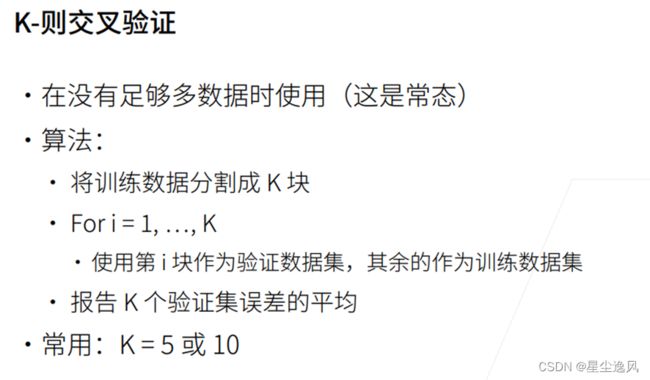
K则交叉验证

正则

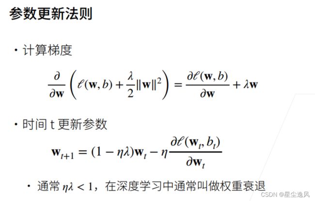
L2正则项实现和所在模型代码的位置如下

训练时 ， l=loss(net(x),y)+lambd*l2_penalty(w)
直接调包 ， trainer=torch.optim.SGD(…，weight_decay=wd) ，这一项

卷积

卷积操作其实就是一种滤波

import torch
from torch import nn
def corr2d(X, K):
    """计算二维互相关运算（卷积）"""
    h, w = K.shape
    Y = torch.zeros((X.shape[0] - h + 1, X.shape[1] - w + 1))
    for i in range(Y.shape[0]):
        for j in range(Y.shape[1]):
            Y[i, j] = (X[i:i + h, j:j + w] * K).sum()
    return Y

class Conv2D(nn.Module):  # 卷积层，传参指定卷积核大小
    def __init__(self, kernel_size):
        super().__init__()
        self.weight = nn.Parameter(torch.rand(kernel_size))
        self.bias = nn.Parameter(torch.zeros(1))

    def forward(self, x):
        return corr2d(x, self.weight) + self.bias

X = torch.ones((6, 8))
X[:, 2:6] = 0
K = torch.tensor([[1.0, -1.0]])
Y = corr2d(X, K)
print(Y)  # 用k矩阵来滤波，边缘检测
# exit()

conv2d = nn.Conv2d(1,1, kernel_size=(1, 2), bias=False)  # 输入输出通道为1，如果是彩色输入通道就是3
# 如加padding=1代表4周都填充一列 ，如加stride=2代表步幅为2

# 使用四维输入和输出格式（批量大小、通道、高度、宽度），其中批量大小和通道数都为1
X = X.reshape((1, 1, 6, 8))
Y = Y.reshape((1, 1, 6, 7))
lr = 3e-2  # 学习率

for i in range(10):
    Y_hat = conv2d(X)
    l = (Y_hat - Y) ** 2
    conv2d.zero_grad()
    l.sum().backward()
    # 迭代卷积核
    conv2d.weight.data[:] -= lr * conv2d.weight.grad  # 手动更新参数，等同于trainer.step()
    if (i + 1) % 2 == 0:
        print(f'epoch {i+1}, loss {l.sum():.3f}')
print(conv2d.weight.data)  # tensor([[[[ 1.0404, -0.9358]]]])，和k的真实值差不多

在感受野相同的情况下，核越小，计算量越小，并且卷积层变成深层后实际上是整张图的视野都有，所以核的大小不是特别重要
越“深”的模型要比“胖”的模型表现更好，同时也具备了更强的非线性，所以，全连接模型的隐藏层小但深的比隐藏层大但浅的好，卷积模型核小但深的比核大但浅的好

一般如果输出大小变小的时候，就会把输出通道变大一些（空间信息压缩 提取到更多的信息单独在更多的通道存下来）

pool2d = nn.MaxPool2d(3, padding=1, stride=2)
pool2d(X)

池化层在卷积层之后，作用是使得卷积不要太对位置信息敏感、减少参数计算量，它没有参数
不过感觉池化用的越来越少了，比如可以用卷积层加stride可以减少参数大小，还有数据增强 图像变换 然后训练，位置信息也就不太需要手动缓解敏感度了

批量归一化BN

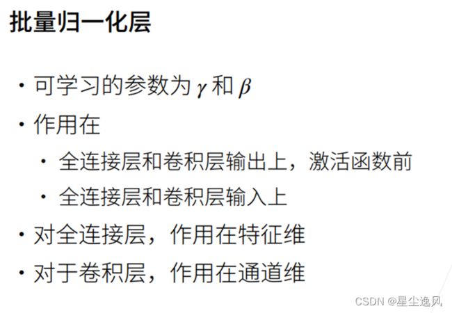
模型训练过程中，批量规范化利用小批量的均值和标准差（有一定的随机性），不断调整神经网络的中间输出，使整个神经网络各层的中间输出值更加稳定
BN层一般用于深层网络，浅层不太需要

实现就是模型层加入比如nn.BatchNorm2d(12)

经典卷积网络

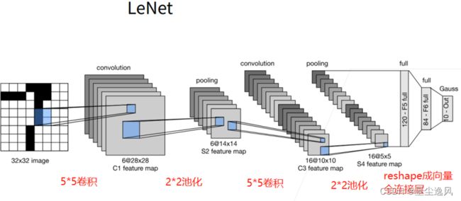
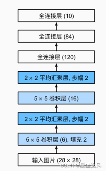
LeNet

import torch
from torch import nn
from torchvision import transforms  # 有各种数据集
import torchvision
from torch.utils import data
net = nn.Sequential(
    nn.Conv2d(1, 6, kernel_size=5, padding=2), nn.Sigmoid(),
    nn.AvgPool2d(kernel_size=2, stride=2),
    nn.Conv2d(6, 16, kernel_size=5), nn.Sigmoid(),
    nn.AvgPool2d(kernel_size=2, stride=2),
    nn.Flatten(),  # 变成1维向量
    nn.Linear(16 * 5 * 5, 120), nn.Sigmoid(),
    nn.Linear(120, 84), nn.Sigmoid(),
    nn.Linear(84, 10))

X = torch.rand(size=(1, 1, 28, 28), dtype=torch.float32)  # 输入是1维28大小的黑白图
for layer in net:
    X = layer(X)
    print(layer.__class__.__name__,'output shape: \t',X.shape)  # 查看每层的形状
    # Conv2d output shape: 	 torch.Size([1, 6, 28, 28])


# 训练过程和前面 后面差不多，可复用
def load_data_fashion_mnist(batch_size, resize=None):
    """下载Fashion-MNIST数据集，然后将其加载到内存中"""
    trans = [transforms.ToTensor()]   # 将图像数据从PIL类型变换成32位浮点数格式，并除以255使得数值在0到1之间
    if resize:
        trans.insert(0, transforms.Resize(resize))
    trans = transforms.Compose(trans)
    mnist_train = torchvision.datasets.FashionMNIST(
        root="../data", train=True, transform=trans, download=True)
    mnist_test = torchvision.datasets.FashionMNIST(
        root="../data", train=False, transform=trans, download=True)
    return (data.DataLoader(mnist_train, batch_size, shuffle=True),
            data.DataLoader(mnist_test, batch_size, shuffle=False))
batch_size = 256
train_iter, test_iter = load_data_fashion_mnist(batch_size=batch_size)


class Accumulator:
    """在n个变量上累加"""
    def __init__(self, n):
        self.data = [0.0] * n
    def add(self, *args):
        self.data = [a + float(b) for a, b in zip(self.data, args)]
    def reset(self):
        self.data = [0.0] * len(self.data)
    def __getitem__(self, idx):
        return self.data[idx]

def accuracy(y_hat, y):
    """计算预测正确的数量"""
    if len(y_hat.shape) > 1 and y_hat.shape[1] > 1:
        y_hat = y_hat.argmax(axis=1)
    cmp = y_hat.type(y.dtype) == y
    return float(cmp.type(y.dtype).sum())

def evaluate_accuracy(net, data_iter):
    """计算在指定数据集上模型的精度"""
    if isinstance(net, torch.nn.Module):
        net.eval()  # 将模型设置为评估模式
    metric = Accumulator(2)  # 正确预测数、预测总数
    with torch.no_grad():
        for X, y in data_iter:
            metric.add(accuracy(net(X), y), y.numel())
    return metric[0] / metric[1]

def train_epoch_ch3(net, train_iter, loss, updater):
    """训练模型一个迭代周期"""
    # 将模型设置为训练模式
    if isinstance(net, torch.nn.Module):
        net.train()
    # 训练损失总和、训练准确度总和、样本数
    metric = Accumulator(3)
    for X, y in train_iter:
        # 计算梯度并更新参数
        y_hat = net(X)
        l = loss(y_hat, y)
        if isinstance(updater, torch.optim.Optimizer):
            # 使用PyTorch内置的优化器和损失函数
            updater.zero_grad()
            l.mean().backward()
            updater.step()
        else:
            # 使用定制的优化器和损失函数
            l.sum().backward()
            updater(X.shape[0])
        metric.add(float(l.sum()), accuracy(y_hat, y), y.numel())
    # 返回训练损失和训练精度
    return metric[0] / metric[2], metric[1] / metric[2]

def train_ch3(net, train_iter, test_iter, loss, num_epochs, updater):
    """训练模型"""
    for epoch in range(num_epochs):
        train_metrics = train_epoch_ch3(net, train_iter, loss, updater)
        test_acc = evaluate_accuracy(net, test_iter)
        print(train_metrics)  # 打印loss和acc，(0.00175, 0.84773)
    train_loss, train_acc = train_metrics
    assert train_loss < 0.5, train_loss
    assert train_acc <= 1 and train_acc > 0.7, train_acc
    assert test_acc <= 1 and test_acc > 0.7, test_acc

def init_weights(m):
    if type(m) == nn.Linear or type(m) == nn.Conv2d:
        nn.init.xavier_uniform_(m.weight)
net.apply(init_weights) # Xavier随机初始化

lr, num_epochs = 0.9, 5
optimizer = torch.optim.SGD(net.parameters(), lr=lr)
loss = nn.CrossEntropyLoss()

train_ch3(net, train_iter, test_iter,loss, num_epochs, optimizer)

AlexNet

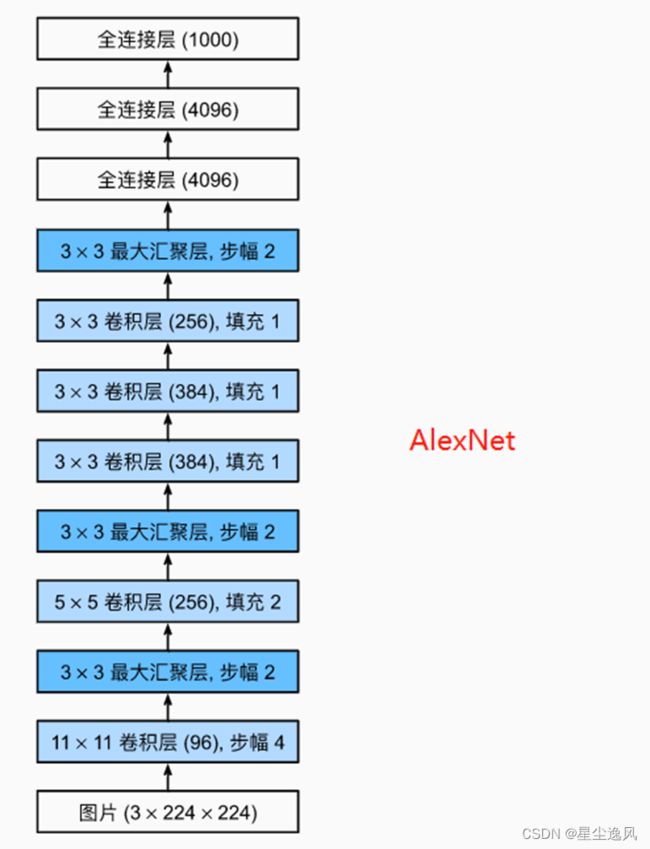
net = nn.Sequential(
    # 这里，我们使用一个11*11的更大窗口来捕捉对象。步幅为4，以减少输出的高度和宽度。
    nn.Conv2d(1, 96, kernel_size=11, stride=4, padding=1), nn.ReLU(),
    nn.MaxPool2d(kernel_size=3, stride=2),
    # 减小卷积窗口，使用填充为2来使得输入与输出的高和宽一致，且增大输出通道数
    nn.Conv2d(96, 256, kernel_size=5, padding=2), nn.ReLU(),
    nn.MaxPool2d(kernel_size=3, stride=2),
    # 使用三个连续的卷积层和较小的卷积窗口。
    # 除了最后的卷积层，输出通道的数量进一步增加。
    # 在前两个卷积层之后，汇聚层不用于减少输入的高度和宽度
    nn.Conv2d(256, 384, kernel_size=3, padding=1), nn.ReLU(),
    nn.Conv2d(384, 384, kernel_size=3, padding=1), nn.ReLU(),
    nn.Conv2d(384, 256, kernel_size=3, padding=1), nn.ReLU(),
    nn.MaxPool2d(kernel_size=3, stride=2),
    nn.Flatten(),
    # 这里，全连接层的输出数量很大。使用dropout层来减轻过拟合
    nn.Linear(6400, 4096), nn.ReLU(),
    nn.Dropout(p=0.5),
    nn.Linear(4096, 4096), nn.ReLU(),
    nn.Dropout(p=0.5),
    nn.Linear(4096, 1000))      # 输出层。类别数1000

VGGNet

视觉几何组（visualgeometry group），VGG块

def vgg_block(num_convs, in_channels, out_channels): # 卷积层数量num_convs、输入通道、输出通道
    layers = []
    for _ in range(num_convs):
        layers.append(nn.Conv2d(in_channels, out_channels,
                                kernel_size=3, padding=1))
        layers.append(nn.ReLU())
        in_channels = out_channels
    layers.append(nn.MaxPool2d(kernel_size=2,stride=2))
    return nn.Sequential(*layers)

# VGG-11
conv_arch = ((1, 64), (1, 128), (2, 256), (2, 512), (2, 512))
def vgg(conv_arch):
    conv_blks = []
    in_channels = 1
    # 卷积层部分
    for (num_convs, out_channels) in conv_arch:
        conv_blks.append(vgg_block(num_convs, in_channels, out_channels))
        in_channels = out_channels

    return nn.Sequential(
        *conv_blks, nn.Flatten(),
        # 全连接层部分
        nn.Linear(out_channels * 7 * 7, 4096), nn.ReLU(), nn.Dropout(0.5),
        nn.Linear(4096, 4096), nn.ReLU(), nn.Dropout(0.5),
        nn.Linear(4096, 10))
net = vgg(conv_arch)

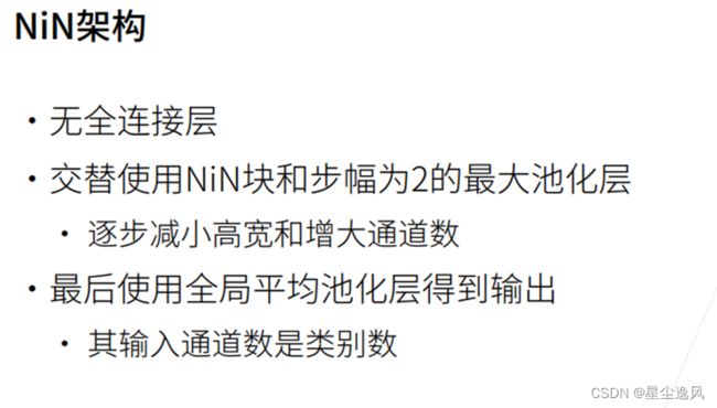
NiN

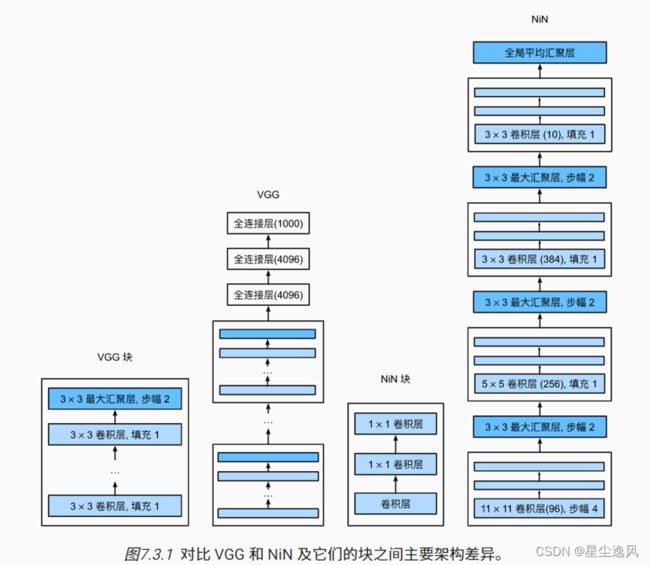
def nin_block(in_channels, out_channels, kernel_size, strides, padding):
    return nn.Sequential(
        nn.Conv2d(in_channels, out_channels, kernel_size, strides, padding),
        nn.ReLU(),
        nn.Conv2d(out_channels, out_channels, kernel_size=1), nn.ReLU(),
        nn.Conv2d(out_channels, out_channels, kernel_size=1), nn.ReLU())

net = nn.Sequential(
    nin_block(1, 96, kernel_size=11, strides=4, padding=0),
    nn.MaxPool2d(3, stride=2),
    nin_block(96, 256, kernel_size=5, strides=1, padding=2),
    nn.MaxPool2d(3, stride=2),
    nin_block(256, 384, kernel_size=3, strides=1, padding=1),
    nn.MaxPool2d(3, stride=2),
    nn.Dropout(0.5),
    # 标签类别数是10
    nin_block(384, 10, kernel_size=3, strides=1, padding=1),
    nn.AdaptiveAvgPool2d((1, 1)),
    # 将四维的输出转成二维的输出，其形状为(批量大小,10)
    nn.Flatten())

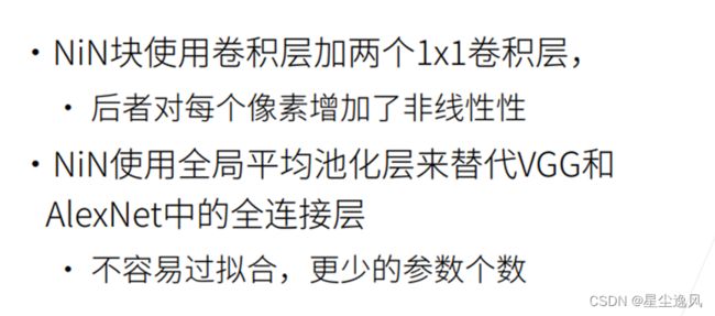
这个模型的效果不算太好，也没有多么增加运算效率，一般用别的
但它的改造思想是很有意义的

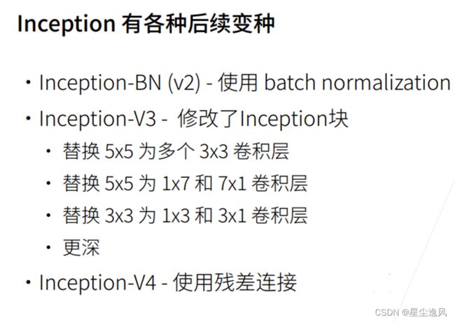
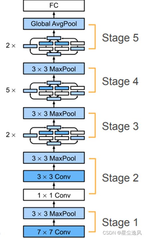
GoogLeNet

GoogleNet的块结构把lenet核alexnet、vggnet、nin的特点都借鉴了，做并行处理，可以使得模型参数变小，并且可以使模型更深

Inception块由四条并行路径组成。
前三条路径使用窗口大小为11、33、5*5的卷积层，不同大小的滤波器可以有效地识别不同范围的图像细节。
中间的两条路径在输入上执行卷积，以减少通道数，降低模型的复杂性。
第四条路径使用最大汇聚层，然后使用卷积层来改变通道数。
这四条路径都使用合适的填充来使输入输出的高宽一致，最后将这四个输出在通道维度上cat作为Inception块的输出。
在Inception块通常调整的超参数是每层输出通道数

from torch.nn import functional as F
class Inception(nn.Module):   # inception块
    # c1--c4是每条路径的输出通道数
    def __init__(self, in_channels, c1, c2, c3, c4, **kwargs):
        super(Inception, self).__init__(**kwargs)
        # 线路1，单1x1卷积层
        self.p1_1 = nn.Conv2d(in_channels, c1, kernel_size=1)
        # 线路2，1x1卷积层后接3x3卷积层
        self.p2_1 = nn.Conv2d(in_channels, c2[0], kernel_size=1)
        self.p2_2 = nn.Conv2d(c2[0], c2[1], kernel_size=3, padding=1)
        # 线路3，1x1卷积层后接5x5卷积层
        self.p3_1 = nn.Conv2d(in_channels, c3[0], kernel_size=1)
        self.p3_2 = nn.Conv2d(c3[0], c3[1], kernel_size=5, padding=2)
        # 线路4，3x3最大汇聚层后接1x1卷积层
        self.p4_1 = nn.MaxPool2d(kernel_size=3, stride=1, padding=1)
        self.p4_2 = nn.Conv2d(in_channels, c4, kernel_size=1)

    def forward(self, x):
        p1 = F.relu(self.p1_1(x))
        p2 = F.relu(self.p2_2(F.relu(self.p2_1(x))))
        p3 = F.relu(self.p3_2(F.relu(self.p3_1(x))))
        p4 = F.relu(self.p4_2(self.p4_1(x)))
        # 在通道维度上连结输出
        return torch.cat((p1, p2, p3, p4), dim=1)

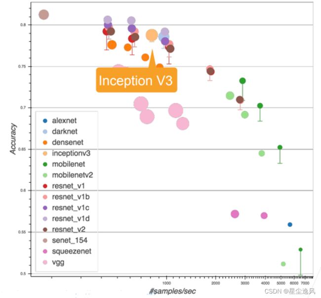
GooleNet比alexnet用了更小的卷积核、更多的通道，在学到的东西不变或变多的基础上，它可以做更深的网络
现在用的少了，一般用inceptionV3、resnet或其他的代替

b1 = nn.Sequential(nn.Conv2d(1, 64, kernel_size=7, stride=2, padding=3),
                   nn.ReLU(),
                   nn.MaxPool2d(kernel_size=3, stride=2, padding=1))

b2 = nn.Sequential(nn.Conv2d(64, 64, kernel_size=1),
                   nn.ReLU(),
                   nn.Conv2d(64, 192, kernel_size=3, padding=1),
                   nn.ReLU(),
                   nn.MaxPool2d(kernel_size=3, stride=2, padding=1))

b3 = nn.Sequential(Inception(192, 64, (96, 128), (16, 32), 32),
                   Inception(256, 128, (128, 192), (32, 96), 64),
                   nn.MaxPool2d(kernel_size=3, stride=2, padding=1))

b4 = nn.Sequential(Inception(480, 192, (96, 208), (16, 48), 64),
                   Inception(512, 160, (112, 224), (24, 64), 64),
                   Inception(512, 128, (128, 256), (24, 64), 64),
                   Inception(512, 112, (144, 288), (32, 64), 64),
                   Inception(528, 256, (160, 320), (32, 128), 128),
                   nn.MaxPool2d(kernel_size=3, stride=2, padding=1))

b5 = nn.Sequential(Inception(832, 256, (160, 320), (32, 128), 128),
                   Inception(832, 384, (192, 384), (48, 128), 128),
                   nn.AdaptiveAvgPool2d((1,1)),
                   nn.Flatten())

net = nn.Sequential(b1, b2, b3, b4, b5, nn.Linear(1024, 10))

ResNet

对于深度神经网络，我们能将新添加的层训练成恒等映射（identity function）f(x)=x，新模型和原模型将同样有效。由于新模型可能得出更优的解来拟合训练数据集，因此添加层似乎更容易降低训练误差。
残差网络的核心思想是：每个附加层都应该更容易地包含原始函数作为其元素之一

f(x)=x+g(x)还一个好处就是如果g(x)的模型没啥用，那它就没梯度，网络就直接f(x)=x过去了,容易训练和优化，加入它也不会使你的模型在目前的基础上变坏

还有很多种不同的残差块，需要实验才知道都怎么样

class Residual(nn.Module):   # 残差块
    def __init__(self, input_channels, num_channels,
                 use_1x1conv=False, strides=1):
        super().__init__()
        self.conv1 = nn.Conv2d(input_channels, num_channels,
                               kernel_size=3, padding=1, stride=strides)
        self.conv2 = nn.Conv2d(num_channels, num_channels,
                               kernel_size=3, padding=1)
        if use_1x1conv:
            self.conv3 = nn.Conv2d(input_channels, num_channels,
                                   kernel_size=1, stride=strides)
        else:
            self.conv3 = None
        self.bn1 = nn.BatchNorm2d(num_channels)
        self.bn2 = nn.BatchNorm2d(num_channels)

    def forward(self, X):
        Y = F.relu(self.bn1(self.conv1(X)))
        Y = self.bn2(self.conv2(Y))
        if self.conv3:
            X = self.conv3(X)
        Y += X   # 精髓，输出再加上输入
        return F.relu(Y)

# 模型结构和vgg、googlenet差不多
b1 = nn.Sequential(nn.Conv2d(1, 64, kernel_size=7, stride=2, padding=3),
                   nn.BatchNorm2d(64), nn.ReLU(),
                   nn.MaxPool2d(kernel_size=3, stride=2, padding=1))

def resnet_block(input_channels, num_channels, num_residuals,
                 first_block=False):
    blk = []
    for i in range(num_residuals):
        if i == 0 and not first_block:
            blk.append(Residual(input_channels, num_channels,
                                use_1x1conv=True, strides=2))
        else:
            blk.append(Residual(num_channels, num_channels))
    return blk

b2 = nn.Sequential(*resnet_block(64, 64, 2, first_block=True))
b3 = nn.Sequential(*resnet_block(64, 128, 2))
b4 = nn.Sequential(*resnet_block(128, 256, 2))
b5 = nn.Sequential(*resnet_block(256, 512, 2))

net = nn.Sequential(b1, b2, b3, b4, b5,
                    nn.AdaptiveAvgPool2d((1,1)),
                    nn.Flatten(), nn.Linear(512, 10))

DenseNet

稠密网络主要由2部分构成：稠密块（dense block）和过渡层（transition layer）
一个稠密块由多个卷积块组成，每个卷积块使用相同的输出通道数，然后把输入和输出在通道维上连结
由于每个稠密块都会带来通道数的增加，使用过多则会过于复杂化模型。而过渡层可以用来控制模型复杂度，它通过1*1卷积层来减小通道数，并使用步幅为2的avgpooling减半高宽，用来降低模型复杂度。

def conv_block(input_channels, num_channels):
    return nn.Sequential(
        nn.BatchNorm2d(input_channels), nn.ReLU(),
        nn.Conv2d(input_channels, num_channels, kernel_size=3, padding=1))

class DenseBlock(nn.Module):
    def __init__(self, num_convs, input_channels, num_channels):
        super(DenseBlock, self).__init__()
        layer = []
        for i in range(num_convs):
            layer.append(conv_block(
                num_channels * i + input_channels, num_channels))
        self.net = nn.Sequential(*layer)

    def forward(self, X):
        for blk in self.net:
            Y = blk(X)
            X = torch.cat((X, Y), dim=1) # 精髓，连接通道维度上每个块的输入和输出
        return X

def transition_block(input_channels, num_channels):  # 过渡层
    return nn.Sequential(
        nn.BatchNorm2d(input_channels), nn.ReLU(),
        nn.Conv2d(input_channels, num_channels, kernel_size=1),
        nn.AvgPool2d(kernel_size=2, stride=2))

稠密连接网络DenseNet，和resnet不同的就是把加的x项直接cat到g(x)里面了
DenseNet同ResNet一样先使用了单卷积层和最大汇聚层，然后上4个可以自定义卷积层的稠密块+过渡层，最后接上全局汇聚层和全连接层来输出结果

# DenseNet模型
b1 = nn.Sequential(
    nn.Conv2d(1, 64, kernel_size=7, stride=2, padding=3),
    nn.BatchNorm2d(64), nn.ReLU(),
    nn.MaxPool2d(kernel_size=3, stride=2, padding=1))

# num_channels为当前的通道数
num_channels, growth_rate = 64, 32
num_convs_in_dense_blocks = [4, 4, 4, 4]
blks = []
for i, num_convs in enumerate(num_convs_in_dense_blocks):
    blks.append(DenseBlock(num_convs, num_channels, growth_rate))
    # 上一个稠密块的输出通道数
    num_channels += num_convs * growth_rate
    # 在稠密块之间添加一个转换层，使通道数量减半
    if i != len(num_convs_in_dense_blocks) - 1:
        blks.append(transition_block(num_channels, num_channels // 2))
        num_channels = num_channels // 2

net = nn.Sequential(
    b1, *blks,
    nn.BatchNorm2d(num_channels), nn.ReLU(),
    nn.AdaptiveAvgPool2d((1, 1)),
    nn.Flatten(),
    nn.Linear(num_channels, 10))

DenseNet可以说是一种隐式的强监督模式，因为每一层都建立起了与前面层的连接，误差信号可以很容易地传播到较早的层，所以较早的层可以从最终分类层获得直接监管
在标准的卷积网络中,最终输出只会利用提取最高层次的特征。而在DenseNet中,它使用了不同层次的特征,它倾向于给出更平滑的决策边界。这也说明了为什么训练数据不足时DenseNet表现依旧良好。

GPU相关

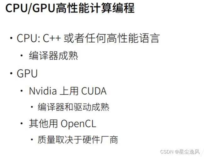
CPU由存储器、控制器和运算器组成，是中央处理器，并不是专用于数值计算，所以难以做高性能计算，性能优化主要看数据读写效率和多线程
GPU是专门针对图形计算而设计的处理器，擅长计算密集型任务，它主要集成了大量的ALU（算术逻辑单元），很擅长并行计算，但没有极其复杂的指令解码器、分支预测等，所以cpu可以做了gpu任务 虽然慢一点，但gpu代替不了cpu（可以类比成cpu是将军 挥斥方遒、gpu是小兵 都是做计算任务的零件 人海战术）

GPU跑AI任务，一般用数据并行，只有模型太大时才用模型并行，多机器GPU训练一般都用数据并行

在cmd键入nvidia-smi查看电脑的gpu和cuda版本

torch.cuda.device_count()  # 查询可用gpu数量
x = torch.tensor([1, 2, 3])
print(x.device)  # 查看张量所在设备
GLOBAL.DEVICE = torch.device("cuda" if torch.cuda.is_available() else "cpu")
net.to(GLOBAL.DEVICE)  # 模型上GPU，如果有的话

def try_gpu(i=0):  
    """如果存在，则返回gpu(i)，否则返回cpu()"""
    if torch.cuda.device_count() >= i + 1:
        return torch.device(f'cuda:{i}')
    return torch.device('cpu')

def try_all_gpus(): 
    """返回所有可用的GPU，如果没有GPU，则返回[cpu(),]"""
    devices = [torch.device(f'cuda:{i}')
             for i in range(torch.cuda.device_count())]
    return devices if devices else [torch.device('cpu')]

try_gpu(), try_gpu(10), try_all_gpus()
(device(type='cuda', index=0),
 device(type='cpu'),
 [device(type='cuda', index=0), device(type='cuda', index=1)])



若想多GPU训练，只需改这两个地方
...
devices = try_all_gpus()
# 模型初始化代码后，在多个GPU上设置模型，框架会自动数据并行
net = nn.DataParallel(net, device_ids=devices)
...
for X, y in train_iter:
    trainer.zero_grad()
    X, y = X.to(devices[0]), y.to(devices[0]) # 训练前，把数据搬到GPU上
    l = loss(net(X), y) # cuda0是主卡，框架会自动把x切到每个gpu上再加起来算loss
    l.backward()
    trainer.step()
...

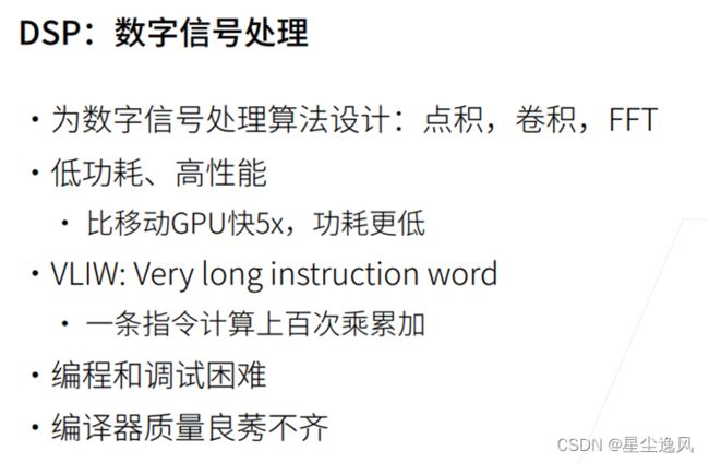
更专用的还有用于数字信号处理的DSP、可编程阵列FPGA 写一堆逻辑单元加法器乘法器等 灵活性高 目前常用、ASIC专用集成电路 为专门目的而设计 灵活性较低 成本较高 研发周期长 所以不太常用

迁移学习

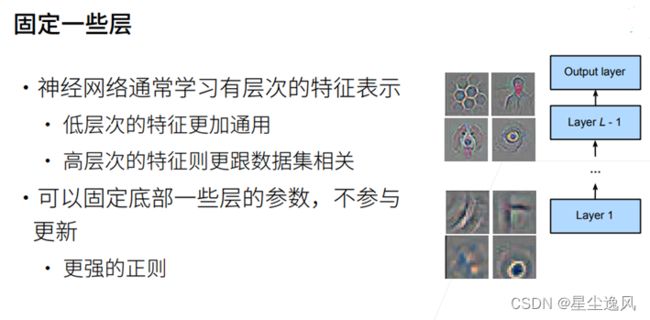
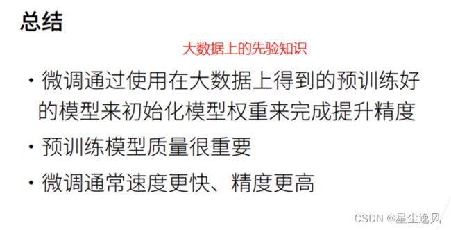
迁移学习，就比如同样做图像分类任务，把一个在imagenet上已经训练好的经典模型如resnet除了输入输出层的特征抽取的层和他们的参数都拿来直接用——作为模型初始化，这样就可以直接从一个提取特征挺厉害的模型开始训练 比模型随机初始化强的不要太多
这就是预训练模型

finetune_net = torchvision.models.resnet18(pretrained=True)  # 加载预训练模型，参数是自动加载预训练的模型参数
print(finetune_net.fc)  # 查看它的输出层，一个linear分类器
finetune_net.fc = nn.Linear(finetune_net.fc.in_features, 2)  # 最后一层改为2分类的分类器
nn.init.xavier_uniform_(finetune_net.fc.weight)  # 只对修改的这层做参数随机初始化

上述代码作为参数初始化的过程，然后就可以直接训练了
trainer = torch.optim.SGD(finetune_net.parameters(), lr=learning_rate)

还有比如以下的做法
pretrained_net = torchvision.models.resnet18(pretrained=True)  # 预训练模型
print(list(pretrained_net.children()))  # 看网络每层的结构
net = nn.Sequential(*list(pretrained_net.children())[:-2])  # 去掉最后的两层不要
net.add_module('final_conv', nn.Conv2d(512, 20, kernel_size=1))  # 接着预训练模型加一层

目标检测

目标检测算法主要分为两个类型
（1）two-stage方法，如R-CNN系算法（region-based CNN），其主要思路是先通过启发式方法（selective search）或者CNN网络（RPN)产生一系列稀疏的候选框，然后对这些候选框进行分类与回归，two-stage方法的优势是准确度高
（2）one-stage方法，如Yolo和SSD，其主要思路是均匀地在图片的不同位置进行密集抽样，抽样时可以采用不同尺度和长宽比，然后利用CNN提取特征后直接进行分类与回归，整个过程只需要一步，所以其优势是速度快，但是均匀的密集采样的一个重要缺点是训练比较困难，这主要是因为正样本与负样本（背景）极其不均衡，导致模型准确度稍低

RCNN、fast RCNN、faster RCNN、mask RCNN

R-CNN对图像选取若干提议区域，使用卷积神经网络对每个提议区域执行前向传播以抽取其特征，然后再用这些特征来预测提议区域的类别和边界框。

RCNN之后，以下这些模型都是为了性能、精度优化一步步提出来的

Fast R-CNN对R-CNN的一个主要改进：只对整个图像做卷积神经网络的前向传播。它还引入了兴趣区域汇聚层，从而为具有不同形状的兴趣区域抽取相同形状的特征。

Faster R-CNN将Fast R-CNN中使用的选择性搜索替换为参与训练的区域提议网络，这样后者可以在减少提议区域数量的情况下仍保证目标检测的精度。

Mask R-CNN在Faster R-CNN的基础上引入了一个全卷积网络，从而借助目标的像素级位置进一步提升目标检测的精度。
它精度高，并且对数据的精度要求也高

SSD

单发多框检测（SSD）
这是一个多尺度目标检测模型，通过多尺度特征块，单发多框检测生成不同大小的锚框，并通过预测边界框的类别和偏移量来检测大小不同的目标（特征金字塔结构）
它先用卷积来抽取图像特征，然后多个卷积层来减小图片大小，在每段都生成锚框 并预测类别和边缘框，顶部段来拟合大物体，底部段拟合小物体

它训练很快，但精度不行

YOLO

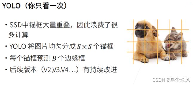
它训练速度很快，但平均精度比faster-RCNN差一点

CenterNet

还有基于非锚框的做法CenterNet，是2019年论文Objects as points中提出，
该网络把目标当成一个点来检测，即用目标box的中心点来表示这个目标，预测目标的中心点偏移量(offset)，宽高(size)来得到物体实际box，而heatmap（热力图）则是表示分类信息
它是速度和精度都比较好，最近研究挺多
https://blog.csdn.net/weixin_42398658/article/details/117514336

SDD实现

定义锚框相关方法

import torch
import torchvision
from torch import nn
from torch.nn import functional as F

# 边界框定义法转换
def box_corner_to_center(boxes):
    """从（左上，右下）转换到（中间，宽度，高度）"""
    x1, y1, x2, y2 = boxes[:, 0], boxes[:, 1], boxes[:, 2], boxes[:, 3]
    cx = (x1 + x2) / 2
    cy = (y1 + y2) / 2
    w = x2 - x1
    h = y2 - y1
    boxes = torch.stack((cx, cy, w, h), axis=-1)
    return boxes

def box_center_to_corner(boxes):
    """从（中间，宽度，高度）转换到（左上，右下）"""
    cx, cy, w, h = boxes[:, 0], boxes[:, 1], boxes[:, 2], boxes[:, 3]
    x1 = cx - 0.5 * w
    y1 = cy - 0.5 * h
    x2 = cx + 0.5 * w
    y2 = cy + 0.5 * h
    boxes = torch.stack((x1, y1, x2, y2), axis=-1)
    return boxes


# 生成锚框的方法
# 指定输入图像、尺寸列表和宽高比列表，然后返回所有的锚框
def multibox_prior(data, sizes, ratios):
    """生成以每个像素为中心具有不同形状的锚框"""
    in_height, in_width = data.shape[-2:]
    device, num_sizes, num_ratios = data.device, len(sizes), len(ratios)
    boxes_per_pixel = (num_sizes + num_ratios - 1)
    size_tensor = torch.tensor(sizes, device=device)
    ratio_tensor = torch.tensor(ratios, device=device)

    # 为了将锚点移动到像素的中心，需要设置偏移量。
    # 因为一个像素的高为1且宽为1，我们选择偏移我们的中心0.5
    offset_h, offset_w = 0.5, 0.5
    steps_h = 1.0 / in_height  # 在y轴上缩放步长
    steps_w = 1.0 / in_width  # 在x轴上缩放步长

    # 生成锚框的所有中心点
    center_h = (torch.arange(in_height, device=device) + offset_h) * steps_h
    center_w = (torch.arange(in_width, device=device) + offset_w) * steps_w
    shift_y, shift_x = torch.meshgrid(center_h, center_w, indexing='ij')
    shift_y, shift_x = shift_y.reshape(-1), shift_x.reshape(-1)

    # 生成“boxes_per_pixel”个高和宽，
    # 之后用于创建锚框的四角坐标(xmin,xmax,ymin,ymax)
    w = torch.cat((size_tensor * torch.sqrt(ratio_tensor[0]),
                   sizes[0] * torch.sqrt(ratio_tensor[1:])))\
                   * in_height / in_width  # 处理矩形输入
    h = torch.cat((size_tensor / torch.sqrt(ratio_tensor[0]),
                   sizes[0] / torch.sqrt(ratio_tensor[1:])))
    # 除以2来获得半高和半宽
    anchor_manipulations = torch.stack((-w, -h, w, h)).T.repeat(
                                        in_height * in_width, 1) / 2

    # 每个中心点都将有“boxes_per_pixel”个锚框，
    # 所以生成含所有锚框中心的网格，重复了“boxes_per_pixel”次
    out_grid = torch.stack([shift_x, shift_y, shift_x, shift_y],
                dim=1).repeat_interleave(boxes_per_pixel, dim=0)
    output = out_grid + anchor_manipulations
    # print(output.unsqueeze(0).shape)
    return output.unsqueeze(0)   # （批量大小，锚框的数量，4）


def box_iou(boxes1, boxes2):
    """计算两个锚框的交并比"""
    box_area = lambda boxes: ((boxes[:, 2] - boxes[:, 0]) *
                              (boxes[:, 3] - boxes[:, 1]))
    # boxes1,boxes2,areas1,areas2的形状:
    # boxes1：(boxes1的数量,4),
    # boxes2：(boxes2的数量,4),
    # areas1：(boxes1的数量,),
    # areas2：(boxes2的数量,)
    areas1 = box_area(boxes1)
    areas2 = box_area(boxes2)
    # inter_upperlefts,inter_lowerrights,inters的形状:
    # (boxes1的数量,boxes2的数量,2)
    inter_upperlefts = torch.max(boxes1[:, None, :2], boxes2[:, :2])
    inter_lowerrights = torch.min(boxes1[:, None, 2:], boxes2[:, 2:])
    inters = (inter_lowerrights - inter_upperlefts).clamp(min=0)
    # inter_areasandunion_areas的形状:(boxes1的数量,boxes2的数量)
    inter_areas = inters[:, :, 0] * inters[:, :, 1]
    union_areas = areas1[:, None] + areas2 - inter_areas
    return inter_areas / union_areas

def assign_anchor_to_bbox(ground_truth, anchors, device, iou_threshold=0.5):
    """将最接近的真实边界框分配给锚框"""
    num_anchors, num_gt_boxes = anchors.shape[0], ground_truth.shape[0]
    # 位于第i行和第j列的元素x_ij是锚框i和真实边界框j的IoU
    jaccard = box_iou(anchors, ground_truth)
    # 对于每个锚框，分配的真实边界框的张量
    anchors_bbox_map = torch.full((num_anchors,), -1, dtype=torch.long,
                                  device=device)
    # 根据阈值，决定是否分配真实边界框
    max_ious, indices = torch.max(jaccard, dim=1)
    anc_i = torch.nonzero(max_ious >= iou_threshold).reshape(-1)
    box_j = indices[max_ious >= iou_threshold]
    anchors_bbox_map[anc_i] = box_j
    col_discard = torch.full((num_anchors,), -1)
    row_discard = torch.full((num_gt_boxes,), -1)
    for _ in range(num_gt_boxes):
        max_idx = torch.argmax(jaccard)
        box_idx = (max_idx % num_gt_boxes).long()
        anc_idx = (max_idx / num_gt_boxes).long()
        anchors_bbox_map[anc_idx] = box_idx
        jaccard[:, box_idx] = col_discard
        jaccard[anc_idx, :] = row_discard
    return anchors_bbox_map


def offset_boxes(anchors, assigned_bb, eps=1e-6):
    """对锚框偏移量的转换"""
    c_anc = box_corner_to_center(anchors)
    c_assigned_bb = box_corner_to_center(assigned_bb)
    offset_xy = 10 * (c_assigned_bb[:, :2] - c_anc[:, :2]) / c_anc[:, 2:]
    offset_wh = 5 * torch.log(eps + c_assigned_bb[:, 2:] / c_anc[:, 2:])
    offset = torch.cat([offset_xy, offset_wh], axis=1)
    return offset

def multibox_target(anchors, labels):
    """使用真实边界框标记锚框"""
    batch_size, anchors = labels.shape[0], anchors.squeeze(0)
    batch_offset, batch_mask, batch_class_labels = [], [], []
    device, num_anchors = anchors.device, anchors.shape[0]
    for i in range(batch_size):
        label = labels[i, :, :]
        anchors_bbox_map = assign_anchor_to_bbox(
            label[:, 1:], anchors, device)
        bbox_mask = ((anchors_bbox_map >= 0).float().unsqueeze(-1)).repeat(
            1, 4)
        # 将类标签和分配的边界框坐标初始化为零
        class_labels = torch.zeros(num_anchors, dtype=torch.long,
                                   device=device)
        assigned_bb = torch.zeros((num_anchors, 4), dtype=torch.float32,
                                  device=device)
        # 使用真实边界框来标记锚框的类别。
        # 如果一个锚框没有被分配，我们标记其为背景（值为零）
        indices_true = torch.nonzero(anchors_bbox_map >= 0)
        bb_idx = anchors_bbox_map[indices_true]
        class_labels[indices_true] = label[bb_idx, 0].long() + 1
        assigned_bb[indices_true] = label[bb_idx, 1:]
        # 偏移量转换
        offset = offset_boxes(anchors, assigned_bb) * bbox_mask
        batch_offset.append(offset.reshape(-1))
        batch_mask.append(bbox_mask.reshape(-1))
        batch_class_labels.append(class_labels)
    bbox_offset = torch.stack(batch_offset)
    bbox_mask = torch.stack(batch_mask)
    class_labels = torch.stack(batch_class_labels)
    return (bbox_offset, bbox_mask, class_labels)


def offset_inverse(anchors, offset_preds):
    """根据带有预测偏移量的锚框来预测边界框"""
    anc = box_corner_to_center(anchors)
    pred_bbox_xy = (offset_preds[:, :2] * anc[:, 2:] / 10) + anc[:, :2]
    pred_bbox_wh = torch.exp(offset_preds[:, 2:] / 5) * anc[:, 2:]
    pred_bbox = torch.cat((pred_bbox_xy, pred_bbox_wh), axis=1)
    predicted_bbox = box_center_to_corner(pred_bbox)
    return predicted_bbox

def nms(boxes, scores, iou_threshold):
    """对预测边界框的置信度进行排序"""
    B = torch.argsort(scores, dim=-1, descending=True)
    keep = []  # 保留预测边界框的指标
    while B.numel() > 0:
        i = B[0]
        keep.append(i)
        if B.numel() == 1: break
        iou = box_iou(boxes[i, :].reshape(-1, 4),
                      boxes[B[1:], :].reshape(-1, 4)).reshape(-1)
        inds = torch.nonzero(iou <= iou_threshold).reshape(-1)
        B = B[inds + 1]
    return torch.tensor(keep, device=boxes.device)

def multibox_detection(cls_probs, offset_preds, anchors, nms_threshold=0.5,
                       pos_threshold=0.009999999):
    """使用非极大值抑制来预测边界框"""
    device, batch_size = cls_probs.device, cls_probs.shape[0]
    anchors = anchors.squeeze(0)
    num_classes, num_anchors = cls_probs.shape[1], cls_probs.shape[2]
    out = []
    for i in range(batch_size):
        cls_prob, offset_pred = cls_probs[i], offset_preds[i].reshape(-1, 4)
        conf, class_id = torch.max(cls_prob[1:], 0)
        predicted_bb = offset_inverse(anchors, offset_pred)
        keep = nms(predicted_bb, conf, nms_threshold)

        # 找到所有的non_keep索引，并将类设置为背景
        all_idx = torch.arange(num_anchors, dtype=torch.long, device=device)
        combined = torch.cat((keep, all_idx))
        uniques, counts = combined.unique(return_counts=True)
        non_keep = uniques[counts == 1]
        all_id_sorted = torch.cat((keep, non_keep))
        class_id[non_keep] = -1
        class_id = class_id[all_id_sorted]
        conf, predicted_bb = conf[all_id_sorted], predicted_bb[all_id_sorted]
        # pos_threshold是一个用于非背景预测的阈值
        below_min_idx = (conf < pos_threshold)
        class_id[below_min_idx] = -1
        conf[below_min_idx] = 1 - conf[below_min_idx]
        pred_info = torch.cat((class_id.unsqueeze(1),
                               conf.unsqueeze(1),
                               predicted_bb), dim=1)
        out.append(pred_info)
    return torch.stack(out)

定义模型

# 类别预测层
# 锚框有目标类别num_classes+1背景 个类别，输入数据以每个单元为中心生成num_anchors个锚框
# 用卷积层的通道来输出类别预测（类别*锚框）
def cls_predictor(num_inputs, num_anchors, num_classes):
    return nn.Conv2d(num_inputs, num_anchors * (num_classes + 1),
                     kernel_size=3, padding=1)

# 边缘框预测层，预测锚框的4个偏移量
def bbox_predictor(num_inputs, num_anchors):
    return nn.Conv2d(num_inputs, num_anchors * 4, kernel_size=3, padding=1)

def flatten_pred(pred):  # 将通道维移到最后一维
    return torch.flatten(pred.permute(0, 2, 3, 1), start_dim=1)
def concat_preds(preds):  # 将预测结果转成二维（批量大小，高*宽*通道）的格式
    return torch.cat([flatten_pred(p) for p in preds], dim=1)
# 这样的话，尽管Y1和Y2在通道数 高 宽是不同大小，仍能在同一个batch的两个不同尺度上连接这两个预测输出，以提高计算效率


# 高宽减半块
def down_sample_blk(in_channels, out_channels):
    blk = []
    for _ in range(2):  # 类VGG块
        blk.append(nn.Conv2d(in_channels, out_channels,
                             kernel_size=3, padding=1))
        blk.append(nn.BatchNorm2d(out_channels))
        blk.append(nn.ReLU())
        in_channels = out_channels
    blk.append(nn.MaxPool2d(2))
    return nn.Sequential(*blk)

# 基本网络块用于从输入图像中抽取特征，高宽减半同时通道翻倍
def base_net():
    blk = []
    num_filters = [3, 16, 32, 64]
    for i in range(len(num_filters) - 1):
        blk.append(down_sample_blk(num_filters[i], num_filters[i+1]))
    return nn.Sequential(*blk)

# 完整的单发多框检测模型由五个模块组成。每个块生成的特征图既用于生成锚框，又用于预测这些锚框的类别和偏移量
# 五个模块中，第一个是基本网络块，第二个到第四个是高和宽减半块，最后一个模块使用全局最大池将高度和宽度都降到1
def get_blk(i):
    if i == 0:
        blk = base_net()
    elif i == 1:
        blk = down_sample_blk(64, 128)
    elif i == 4:
        blk = nn.AdaptiveMaxPool2d((1,1))
    else:
        blk = down_sample_blk(128, 128)
    return blk



# 定义前向传播
# 与图像分类不同，它的输出是：CNN特征图Y；在当前尺度下根据Y生成的锚框；预测的这些锚框的类别和偏移量（基于Y）
def blk_forward(X, blk, size, ratio, cls_predictor, bbox_predictor):
    Y = blk(X)
    anchors = multibox_prior(Y, sizes=size, ratios=ratio)
    cls_preds = cls_predictor(Y)
    bbox_preds = bbox_predictor(Y)
    # print('blk shape',(Y.shape, anchors.shape, cls_preds.shape, bbox_preds.shape))
    return (Y, anchors, cls_preds, bbox_preds)


# 根据实际情况统计分析 来设置锚框的比例大小的超参数
sizes = [[0.2, 0.272], [0.37, 0.447], [0.54, 0.619], [0.71, 0.79],
         [0.88, 0.961]]  # 每层锚框的大小比例
ratios = [[1, 2, 0.5]] * 5   # 锚框的选择范围
num_anchors = len(sizes[0]) + len(ratios[0]) - 1
class TinySSD(nn.Module):
    def __init__(self, num_classes, **kwargs):
        super(TinySSD, self).__init__(**kwargs)
        self.num_classes = num_classes
        idx_to_in_channels = [64, 128, 128, 128, 128]
        for i in range(5):
            # 即赋值语句self.blk_i=get_blk(i)
            setattr(self, f'blk_{i}', get_blk(i))
            setattr(self, f'cls_{i}', cls_predictor(idx_to_in_channels[i],
                                                    num_anchors, num_classes))
            setattr(self, f'bbox_{i}', bbox_predictor(idx_to_in_channels[i],
                                                      num_anchors))

    def forward(self, X):  # 卷积一直往下走，但最后只每次取出检测锚框的东西，卷积出来的结果不需要
        anchors, cls_preds, bbox_preds = [None] * 5, [None] * 5, [None] * 5
        for i in range(5):
            # getattr(self,'blk_%d'%i)即访问self.blk_i
            X, anchors[i], cls_preds[i], bbox_preds[i] = blk_forward(
                X, getattr(self, f'blk_{i}'), sizes[i], ratios[i],
                getattr(self, f'cls_{i}'), getattr(self, f'bbox_{i}'))
        # 5层金字塔结构，对每一层做前向传播，最后cat合并
        anchors = torch.cat(anchors, dim=1)
        cls_preds = concat_preds(cls_preds)
        cls_preds = cls_preds.reshape(
            cls_preds.shape[0], -1, self.num_classes + 1)
        bbox_preds = concat_preds(bbox_preds)
        return anchors, cls_preds, bbox_preds


net = TinySSD(num_classes=1)  # 两类问题
X = torch.zeros((32, 3, 256, 256))  # 32批量，3通道RGB，256图片大小
anchors, cls_preds, bbox_preds = net(X)

# 以图像每个单元为中心有4个锚框生成 num_anchors为4，乘上卷积后的图片大小32*32...4096+1024+256+64+4
print('output anchors:', anchors.shape) # torch.Size([1, 5444, 4])
# sum（锚框数4*类别数2*大小 / 预测类别数的2）
print('output class preds:', cls_preds.shape) # torch.Size([32, 5444, 2])
# sum 锚框的偏移，并转成二维（批量，高*宽*通道）
print('output bbox preds:', bbox_preds.shape) #  torch.Size([32, 21776])

加载训练数据集

import os
import pandas as pd
from d2l import torch as d2l

def read_data_bananas(is_train=True):
    """读取香蕉检测数据集中的图像和标签"""
    data_dir = d2l.download_extract('banana-detection')
    csv_fname = os.path.join(data_dir, 'bananas_train' if is_train
                             else 'bananas_val', 'label.csv')
    csv_data = pd.read_csv(csv_fname)
    csv_data = csv_data.set_index('img_name')
    images, targets = [], []
    for img_name, target in csv_data.iterrows():
        images.append(torchvision.io.read_image(
            os.path.join(data_dir, 'bananas_train' if is_train else
                         'bananas_val', 'images', f'{img_name}')))
        # 这里的target包含（类别，左上角x，左上角y，右下角x，右下角y），
        # 其中所有图像都具有相同的香蕉类（索引为0）
        targets.append(list(target))
    return images, torch.tensor(targets).unsqueeze(1) / 256
    
class BananasDataset(torch.utils.data.Dataset):
    """一个用于加载香蕉检测数据集的自定义数据集"""
    def __init__(self, is_train):
        self.features, self.labels = read_data_bananas(is_train)
        print('read ' + str(len(self.features)) + (f' training examples' if
              is_train else f' validation examples'))

    def __getitem__(self, idx):
        return (self.features[idx].float(), self.labels[idx])

    def __len__(self):
        return len(self.features)
        
def load_data_bananas(batch_size):
    """加载香蕉检测数据集"""
    train_iter = torch.utils.data.DataLoader(BananasDataset(is_train=True),
                                             batch_size, shuffle=True)
    val_iter = torch.utils.data.DataLoader(BananasDataset(is_train=False),
                                           batch_size)
    return train_iter, val_iter
    
batch_size = 32
train_iter, _ = load_data_bananas(batch_size)
# print(train_iter)

训练代码
目标检测有两种类型的损失，相加得到模型的最终损失函数
第一是有关锚框类别的损失：和图像分类问题里一直用的交叉熵损失函数一样
第二是有关正类锚框偏移量的损失：预测偏移量是一个回归问题。这里用l1范数损失，预测值和真实值之差的绝对值

def try_gpu(i=0):
    if torch.cuda.device_count() >= i + 1:
        return torch.device(f'cuda:{i}')
    return torch.device('cpu')
device, net = try_gpu(), TinySSD(num_classes=1)
# print(device)
trainer = torch.optim.SGD(net.parameters(), lr=0.2, weight_decay=5e-4)

# 目标检测有两种类型的损失，相加得到模型的最终损失函数
# 第一是有关锚框类别的损失：和图像分类问题里一直用的交叉熵损失函数一样
# 第二是有关正类锚框偏移量的损失：预测偏移量是一个回归问题。这里用l1范数损失，预测值和真实值之差的绝对值
cls_loss = nn.CrossEntropyLoss(reduction='none')
bbox_loss = nn.L1Loss(reduction='none')

def calc_loss(cls_preds, cls_labels, bbox_preds, bbox_labels, bbox_masks):
    batch_size, num_classes = cls_preds.shape[0], cls_preds.shape[2]
    cls = cls_loss(cls_preds.reshape(-1, num_classes),
                   cls_labels.reshape(-1)).reshape(batch_size, -1).mean(dim=1)
    bbox = bbox_loss(bbox_preds * bbox_masks,
                     bbox_labels * bbox_masks).mean(dim=1)
    return cls + bbox

# 使用平均绝对误差来评价边界框的预测结果
def cls_eval(cls_preds, cls_labels):
    # 由于类别预测结果放在最后一维，argmax需要指定最后一维。
    return float((cls_preds.argmax(dim=-1).type(
        cls_labels.dtype) == cls_labels).sum())

def bbox_eval(bbox_preds, bbox_labels, bbox_masks):
    return float((torch.abs((bbox_labels - bbox_preds) * bbox_masks)).sum())



# ————

# 训练模型的过程，先在模型的前向传播过程中生成多尺度锚框（anchors），并预测其类别（cls_preds）和偏移量（bbox_preds）
# 然后，根据标签Y为生成的锚框标记类别（cls_labels）和偏移量（bbox_labels）
# 最后，根据类别和偏移量的预测和标注值计算损失函数
num_epochs, timer = 3, d2l.Timer()
animator = d2l.Animator(xlabel='epoch', xlim=[1, num_epochs],
                        legend=['class error', 'bbox mae'])
net = net.to(device)
for epoch in range(num_epochs):
    print('do',epoch)
    # 训练精确度的和，训练精确度的和中的示例数
    # 绝对误差的和，绝对误差的和中的示例数
    metric = d2l.Accumulator(4)
    net.train()
    for features, target in train_iter:
        timer.start()
        trainer.zero_grad()
        X, Y = features.to(device), target.to(device)
        # 生成多尺度的锚框，为每个锚框预测类别和偏移量
        anchors, cls_preds, bbox_preds = net(X)
        # 为每个锚框标注类别和偏移量
        bbox_labels, bbox_masks, cls_labels = multibox_target(anchors, Y)
        # 根据类别和偏移量的预测和标注值计算损失函数
        l = calc_loss(cls_preds, cls_labels, bbox_preds, bbox_labels,
                      bbox_masks)
        l.mean().backward()
        trainer.step()
        metric.add(cls_eval(cls_preds, cls_labels), cls_labels.numel(),
                   bbox_eval(bbox_preds, bbox_labels, bbox_masks),
                   bbox_labels.numel())
    cls_err, bbox_mae = 1 - metric[0] / metric[1], metric[2] / metric[3]
    animator.add(epoch + 1, (cls_err, bbox_mae))
print(f'class err {cls_err:.2e}, bbox mae {bbox_mae:.2e}')   # class err 4.85e-03, bbox mae 5.02e-03
print(f'{len(train_iter.dataset) / timer.stop():.1f} examples/sec on '
      f'{str(device)}')  # 1839.6 examples/sec on cpu

torch.save(net.state_dict(), 'mlp.params')  # 保存模型参数到文件

预测代码

net1 = TinySSD(num_classes=1)  # 声明模型的构造
net1.load_state_dict(torch.load('mlp.params')) # 加载参数到模型中
net1.eval()  # 停止反向传播

from matplotlib import pyplot as plt

X = torchvision.io.read_image('D:\code2022\\new2022\data\\banana-detection\\bananas_train\images\\623.png').unsqueeze(0).float()
img = X.squeeze(0).permute(1, 2, 0).long()


def predict(X):
    # net1.eval()
    anchors, cls_preds, bbox_preds = net1(X.to(device))
    cls_probs = F.softmax(cls_preds, dim=2).permute(0, 2, 1)
    output = multibox_detection(cls_probs, bbox_preds, anchors)
    idx = [i for i, row in enumerate(output[0]) if row[0] != -1]
    return output[0, idx]
output = predict(X)



def bbox_to_rect(bbox, color):
    return plt.Rectangle(
        xy=(bbox[0], bbox[1]), width=bbox[2]-bbox[0], height=bbox[3]-bbox[1],
        fill=False, edgecolor=color, linewidth=2)
def show_bboxes(axes, bboxes, labels=None, colors=None):
    """显示所有边界框"""
    def _make_list(obj, default_values=None):
        if obj is None:
            obj = default_values
        elif not isinstance(obj, (list, tuple)):
            obj = [obj]
        return obj

    labels = _make_list(labels)
    colors = _make_list(colors, ['b', 'g', 'r', 'm', 'c'])
    for i, bbox in enumerate(bboxes):
        color = colors[i % len(colors)]
        rect = bbox_to_rect(bbox.detach().numpy(), color)
        axes.add_patch(rect)
        if labels and len(labels) > i:
            text_color = 'k' if color == 'w' else 'w'
            axes.text(rect.xy[0], rect.xy[1], labels[i],
                      va='center', ha='center', fontsize=9, color=text_color,
                      bbox=dict(facecolor=color, lw=0))


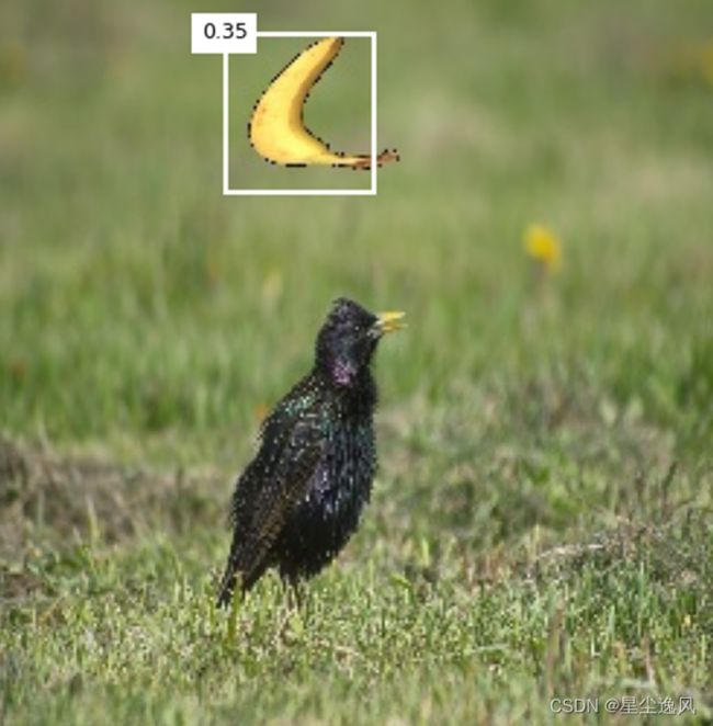
def display(img, output, threshold):
    # d2l.set_figsize((5, 5))
    fig = plt.imshow(img)
    print(output)
    for row in output:
        score = float(row[1])
        if score < threshold:
            continue
        print(1)
        h, w = img.shape[0:2]
        bbox = [row[2:6] * torch.tensor((w, h, w, h), device=row.device)]
        show_bboxes(fig.axes, bbox, '%.2f' % score, 'w')
    plt.show()

display(img, output.cpu(), threshold=0.3)

#YOLO实践

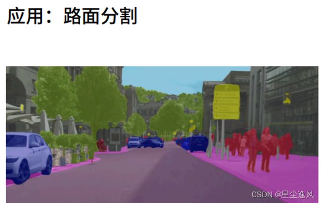
语义分割

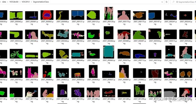
语义分割可以识别并理解图像中每一个像素的内容，语义区域的标注和预测是像素级的
与目标检测相比，语义分割标注的像素级的边框显然更加精细。它广泛应用于医学图像识别、自动驾驶、地质勘探、拍照处理等领域

cv里还有2个与语义分割相似的名词，图像分割（image segmentation）和实例分割（instance segmentation）
图像分割将图像划分为若干组成区域，它的方法通常利用图像中像素之间的相关性。它在训练时不需要有关图像像素的标签信息，在预测时也无法保证分割出的区域具有我们希望得到的语义。
实例分割也叫同时检测并分割（simultaneous detection and segmentation），它研究如何识别图像中各个目标实例的像素级区域。与语义分割不同，实例分割不仅需要区分语义，还要区分不同的目标实例。例如，如果图像中有两条狗，则实例分割需要区分像素属于的两条狗中的哪一条。

转置卷积

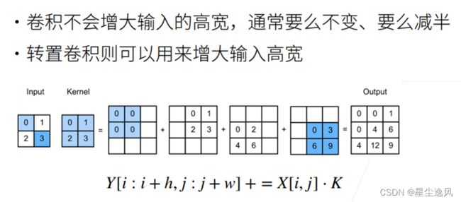
转置卷积的上采样方式并非预设的插值方法，而是同卷积一样，具有可学习的参数，可通过网络学习来获取最优的上采样方式。
它可以用在很多地方，比如
小图像放大-AI修复，用转置卷积学到合适的补全图片的参数
在CAE卷积自编码，卷积用来提取图像特征，转置卷积用来还原特征，编码解码的过程
在DCGAN，生成器将随机值转变为一个全尺寸图片，此时需用到转置卷积
在语义分割，会在编码器中用卷积层提取特征，然后在解码器（用到转置卷积）中恢复原先尺寸，从而对原图中的每个像素分类。经典方法有FCN和U-net。
在CNN可视化，通过转置卷积将CNN的特征图还原到像素空间，以观察特定特征图对哪些模式的图像敏感。
等

def trans_conv(X, K):  # 转置卷积
    h, w = K.shape
    Y = torch.zeros((X.shape[0] + h - 1, X.shape[1] + w - 1))
    for i in range(X.shape[0]):
        for j in range(X.shape[1]):
            Y[i: i + h, j: j + w] += X[i, j] * K
    return Y

# 转置卷积torch实现
tconv = nn.ConvTranspose2d(1, 1, kernel_size=2, bias=False)

FCN

FCN实现

获取和处理数据集

import torch
import torchvision
from torch import nn
from torch.nn import functional as F
from d2l import torch as d2l
from matplotlib import pyplot as plt
import os

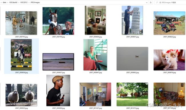
#  最重要的语义分割数据集之一是Pascal VOC2012
# d2l.DATA_HUB['voc2012'] = (d2l.DATA_URL + 'VOCtrainval_11-May-2012.tar',
#                            '4e443f8a2eca6b1dac8a6c57641b67dd40621a49')
# voc_dir = d2l.download_extract('voc2012', 'VOCdevkit/VOC2012')

def read_voc_images(voc_dir, is_train=True):
    """读取所有VOC图像并标注"""
    txt_fname = os.path.join(voc_dir, 'ImageSets', 'Segmentation',
                             'train.txt' if is_train else 'val.txt')
    mode = torchvision.io.image.ImageReadMode.RGB
    with open(txt_fname, 'r') as f:
        images = f.read().split()
    features, labels = [], []
    for i, fname in enumerate(images):
        features.append(torchvision.io.read_image(os.path.join(
            voc_dir, 'JPEGImages', f'{fname}.jpg')))
        labels.append(torchvision.io.read_image(os.path.join(
            voc_dir, 'SegmentationClass' ,f'{fname}.png'), mode))
    return features[:200], labels[:200]  # 因为数据有点多有点卡，现只取200张，就这也不快
train_features, train_labels = read_voc_images('../data/VOCdevkit/VOC2012', True)

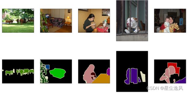
# 画出5张样例对应label看看
n = 5
imgs = train_features[0+33:n+33] + train_labels[0+33:n+33]
imgs = [img.permute(1,2,0) for img in imgs]
def show_images(imgs, num_rows, num_cols, titles=None, scale=1.5):
    figsize = (num_cols * scale, num_rows * scale)
    _, axes = d2l.plt.subplots(num_rows, num_cols, figsize=figsize)
    axes = axes.flatten()
    for i, (ax, img) in enumerate(zip(axes, imgs)):
        if torch.is_tensor(img):
            # Tensor Image
            ax.imshow(img.numpy())
        else:
            # PIL Image
            ax.imshow(img)
        ax.axes.get_xaxis().set_visible(False)
        ax.axes.get_yaxis().set_visible(False)
        if titles:
            ax.set_title(titles[i])
    plt.show()
    return axes
show_images(imgs, 2, n)


# 数据集的索引
VOC_COLORMAP = [[0, 0, 0], [128, 0, 0], [0, 128, 0], [128, 128, 0],
                [0, 0, 128], [128, 0, 128], [0, 128, 128], [128, 128, 128],
                [64, 0, 0], [192, 0, 0], [64, 128, 0], [192, 128, 0],
                [64, 0, 128], [192, 0, 128], [64, 128, 128], [192, 128, 128],
                [0, 64, 0], [128, 64, 0], [0, 192, 0], [128, 192, 0],
                [0, 64, 128]]
VOC_CLASSES = ['background', 'aeroplane', 'bicycle', 'bird', 'boat',
               'bottle', 'bus', 'car', 'cat', 'chair', 'cow',
               'diningtable', 'dog', 'horse', 'motorbike', 'person',
               'potted plant', 'sheep', 'sofa', 'train', 'tv/monitor']
def voc_colormap2label():
    """构建从RGB到VOC类别索引的映射"""
    colormap2label = torch.zeros(256 ** 3, dtype=torch.long)
    for i, colormap in enumerate(VOC_COLORMAP):
        colormap2label[
            (colormap[0] * 256 + colormap[1]) * 256 + colormap[2]] = i
    return colormap2label
def voc_label_indices(colormap, colormap2label):
    """将VOC标签中的RGB值映射到它们的类别索引"""
    colormap = colormap.permute(1, 2, 0).numpy().astype('int32')
    idx = ((colormap[:, :, 0] * 256 + colormap[:, :, 1]) * 256
           + colormap[:, :, 2])
    return colormap2label[idx]


def voc_rand_crop(feature, label, height, width):
    """随机裁剪特征和标签图像"""
    rect = torchvision.transforms.RandomCrop.get_params(
        feature, (height, width))  # 随机裁剪的参数，同时作用到原始图像和label，保持一致
    feature = torchvision.transforms.functional.crop(feature, *rect)
    label = torchvision.transforms.functional.crop(label, *rect)
    return feature, label

class VOCSegDataset(torch.utils.data.Dataset):
    """一个用于加载VOC数据集的自定义数据集"""

    def __init__(self, is_train, crop_size, voc_dir):
        self.transform = torchvision.transforms.Normalize(
            mean=[0.485, 0.456, 0.406], std=[0.229, 0.224, 0.225])
        self.crop_size = crop_size
        features, labels = read_voc_images(voc_dir, is_train=is_train)
        self.features = [self.normalize_image(feature)
                         for feature in self.filter(features)]
        self.labels = self.filter(labels)
        self.colormap2label = voc_colormap2label()
        print('read ' + str(len(self.features)) + ' examples')

    def normalize_image(self, img):   # 对输入图像的RGB三个通道的值分别做标准化
        return self.transform(img.float() / 255)

    def filter(self, imgs):
        return [img for img in imgs if (
            img.shape[1] >= self.crop_size[0] and
            img.shape[2] >= self.crop_size[1])]

    def __getitem__(self, idx):
        feature, label = voc_rand_crop(self.features[idx], self.labels[idx],
                                       *self.crop_size)
        return (feature, voc_label_indices(label, self.colormap2label))

    def __len__(self):
        return len(self.features)

def load_data_voc(batch_size, crop_size):
    """加载VOC语义分割数据集"""
    voc_dir = d2l.download_extract('voc2012', os.path.join(
        'VOCdevkit', 'VOC2012'))
    num_workers = d2l.get_dataloader_workers()
    train_iter = torch.utils.data.DataLoader(
        VOCSegDataset(True, crop_size, voc_dir), batch_size,
        shuffle=True, drop_last=True, num_workers=num_workers)
    test_iter = torch.utils.data.DataLoader(
        VOCSegDataset(False, crop_size, voc_dir), batch_size,
        drop_last=True, num_workers=num_workers)
    return train_iter, test_iter
    
# crop_size = (320, 480)  # 统一输入输出图像大小
# batch_size = 64
# print(load_data_voc(batch_size, crop_size))

# exit()

定义FCN，训练

pretrained_net = torchvision.models.resnet18(pretrained=True)  # 预训练模型
print(list(pretrained_net.children()))  # 看网络每层的结构
net = nn.Sequential(*list(pretrained_net.children())[:-2])  # 去掉最后的全局池化和全连接不要
X = torch.rand(size=(1, 3, 320, 480))
print(net(X).shape)  # ([1, 512, 10, 15])  看采用的预训练模型的输入输出变化，图片大小减了32倍
num_classes = 21
net.add_module('final_conv', nn.Conv2d(512, num_classes, kernel_size=1))  # 先加个1*1卷积吧通道数变成类别数，或比类别数大点也行，就是降低通道好计算
net.add_module('transpose_conv', nn.ConvTranspose2d(num_classes, num_classes,
                                    kernel_size=64, padding=16, stride=32))  # 然后一层转置卷积到原来图片大小



def bilinear_kernel(in_channels, out_channels, kernel_size):  # 双线性插值
    factor = (kernel_size + 1) // 2
    if kernel_size % 2 == 1:
        center = factor - 1
    else:
        center = factor - 0.5
    og = (torch.arange(kernel_size).reshape(-1, 1),
          torch.arange(kernel_size).reshape(1, -1))
    filt = (1 - torch.abs(og[0] - center) / factor) * \
           (1 - torch.abs(og[1] - center) / factor)
    weight = torch.zeros((in_channels, out_channels,
                          kernel_size, kernel_size))
    weight[range(in_channels), range(out_channels), :, :] = filt
    return weight
W = bilinear_kernel(num_classes, num_classes, 64)
net.transpose_conv.weight.data.copy_(W)  # 用双线性插值对转置卷积做初始化


def loss(inputs, targets):  # loss等于所有像素的交叉熵均值
    return F.cross_entropy(inputs, targets, reduction='none').mean(1).mean(1)

num_epochs, lr, wd, devices = 3, 0.001, 1e-3, d2l.try_all_gpus()
trainer = torch.optim.SGD(net.parameters(), lr=lr, weight_decay=wd)

batch_size, crop_size = 32, (320, 480)
train_iter, test_iter = load_data_voc(batch_size, crop_size)
d2l.train_ch13(net, train_iter, test_iter, loss, trainer, num_epochs, devices)  # 和SSD里一样的训练for loop
torch.save(net.state_dict(), 'mlp.params-FCN')  # 保存模型参数到文件

预测代码

net.load_state_dict(torch.load('mlp.params-FCN')) # 加载参数到模型中
net.eval()

def predict(img):
    X = test_iter.dataset.normalize_image(img).unsqueeze(0)  # 输入图像做标准化
    pred = net(X.to(devices[0])).argmax(dim=1)
    return pred.reshape(pred.shape[1], pred.shape[2])

def label2image(pred):  # 将预测类别映射回数据集中的标注颜色
    colormap = torch.tensor(d2l.VOC_COLORMAP, device=devices[0])
    X = pred.long()
    return colormap[X, :]


voc_dir = d2l.download_extract('voc2012', 'VOCdevkit/VOC2012')
test_images, test_labels = d2l.read_voc_images(voc_dir, False)
n, imgs = 4, []
for i in range(n):
    crop_rect = (0, 0, 320, 480)
    X = torchvision.transforms.functional.crop(test_images[i], *crop_rect) # 截取固定大小的图像
    pred = label2image(predict(X))   # 做预测
    imgs += [X.permute(1,2,0), pred.cpu(),
             torchvision.transforms.functional.crop(
                 test_labels[i], *crop_rect).permute(1,2,0)]


def show_images(imgs, num_rows, num_cols, titles=None, scale=1.5):
    figsize = (num_cols * scale, num_rows * scale)
    _, axes = d2l.plt.subplots(num_rows, num_cols, figsize=figsize)
    axes = axes.flatten()
    for i, (ax, img) in enumerate(zip(axes, imgs)):
        if torch.is_tensor(img):
            # Tensor Image
            ax.imshow(img.numpy())
        else:
            # PIL Image
            ax.imshow(img)
        ax.axes.get_xaxis().set_visible(False)
        ax.axes.get_yaxis().set_visible(False)
        if titles:
            ax.set_title(titles[i])
    plt.show()
    return axes
    
show_images(imgs[::3] + imgs[1::3] + imgs[2::3], 3, n, scale=2)

#风格迁移

---

文章太长了有点卡了，接下来的见下节