《动手学深度学习》tensorflow2.0版 第三章笔记
《动手学深度学习》tensorflow2.0版 第三章笔记
-
-
-
- 线性回归训练
- 图像分类数据集(Fashion-MNIST)
- 训练误差(training error)和泛化误差(generalization error)。
- Tensorflow2函数接口说明
-
- GradientTape
- reduce_sum()
- tf.cast()
- tf.concat()
- tf.Variable()
- 广播机制
- tf.gather(params,indices,axis=0 )
- tf.assign()
-
-
花了大半天的时间,学习了下第三章深度学习基础,作为一名tensorflow新手,用最基本的函数去完成一些任务是必要的,否则上来就用更高级接口总会有种外强中干的感觉。即使现在pytorch如日中天,还是认为目前一段时间工业界对tensorflow的需求还是会有很多,但是鄙人特别擅长反向押宝。文中的代码没有实测运行。
本文来自 https://trickygo.github.io/Dive-into-DL-TensorFlow2.0/#/chapter03_DL-basics/3.1_linear-regression
线性回归训练
只利用Tensor和GradientTape来实现一个线性回归的训练
%matplotlib inline
import tensorflow as tf
print(tf.__version__)
from matplotlib import pyplot as plt
import random

    2.0.0

#########

num_inputs = 2
num_examples = 1000
# 训练数据集样本数为1000,输入个数(特征数)为2
true_w = [2, -3.4]
true_b = 4.2
#真实权重和偏差
features = tf.random.normal((num_examples, num_inputs),stddev = 1)
#随机生成的批量样本
labels = true_w[0] * features[:,0] + true_w[1] * features[:,1] + true_b
labels += tf.random.normal(labels.shape,stddev=0.01)
#噪声项服从均值为0、标准差为0.01的正态分布
print(features[0], labels[0])
输出:
(,
 )
通过生成第二个特征features[:, 1]和标签 labels 的散点图,可以更直观地观察两者间的线性关系。
def set_figsize(figsize=(3.5, 2.5)):
    plt.rcParams['figure.figsize'] = figsize

set_figsize()
plt.scatter(features[:, 1], labels, 1)
在训练模型的时候,我们需要遍历数据集并不断读取小批量数据样本。这里我们定义一个函数:它每次返回batch_size(批量大小)个随机样本的特征和标签。
def data_iter(batch_size, features, labels):
    num_examples = len(features)
    indices = list(range(num_examples))
    random.shuffle(indices)
    for i in range(0, num_examples, batch_size):
	# i 在[0,num_examples)范围内,以batch_size递增
        j = indices[i: min(i+batch_size, num_examples)]
		#j在每个batch_size范围内变化,min()此处防止超出最大索引
        yield tf.gather(features, axis=0, indices=j), tf.gather(labels, axis=0, indices=j)
		# yield 看做return之后再把它看做一个是生成器(generator)的一部分(带yield的函数才是真正的迭代器)
		# tf.gather()
让我们读取第一个小批量数据样本并打印。每个批量的特征形状为(10, 2),分别对应批量大小和输入个数;标签形状为批量大小。
batch_size = 10

for X, y in data_iter(batch_size, features, labels):
    print(X, y)
    break
输出:
tf.Tensor(
[[ 0.04718596 -1.5959413 ]
 [ 0.3889716  -1.5288432 ]
 [-1.8489572   1.66422   ]
 [-1.3978077  -0.85818154]
 [-0.36940867 -0.619267  ]
 [-0.15660426  1.1231796 ]
 [ 0.89411694  1.5499148 ]
 [ 1.9971682  -0.56981105]
 [-2.1852891   0.18805206]
 [ 1.3222371  -1.0301086 ]], shape=(10, 2), dtype=float32) tf.Tensor(
[ 9.738684   10.164594   -5.15065     4.3305573   5.568048    0.06494669
  0.7251317  10.128626   -0.8036391  10.343082  ], shape=(10,), dtype=float32)
初始化模型参数
w = tf.Variable(tf.random.normal((num_inputs, 1), stddev=0.01))
b = tf.Variable(tf.zeros((1,)))
定义模型
def linreg(X, w, b):
    return tf.matmul(X, w) + b
定义损失函数
def squared_loss(y_hat, y):
    return (y_hat - tf.reshape(y, y_hat.shape)) ** 2 /2
定义优化算法(小批量随机梯度下降算法)
它通过不断迭代模型参数来优化损失函数。这里自动求梯度模块计算得来的梯度是一个批量样本的梯度和。我们将它除以批量大小来得到平均值。
def sgd(params, lr, batch_size, grads):
    """Mini-batch stochastic gradient descent."""
    for i, param in enumerate(params):
        param.assign_sub(lr * grads[i] / batch_size)
		# tf.assign_sub(ref, value),变量 ref 减去 value值,即 ref = ref - value
训练模型
在训练中,我们将多次迭代模型参数。在每次迭代中,我们根据当前读取的小批量数据样本(特征X和标签y),通过调用反向函数t.gradients计算小批量随机梯度,并调用优化算法sgd迭代模型参数。由于我们之前设批量大小batch_size为10,每个小批量的损失 l l l的形状为(10, 1)。回忆一下自动求梯度一节。由于变量 l l l 并不是一个标量,所以我们可以调用reduce_sum()将其求和得到一个标量,再运行t.gradients得到该变量有关模型参数的梯度。注意在每次更新完参数后不要忘了将参数的梯度清零。
在一个迭代周期(epoch)中,我们将完整遍历一遍data_iter函数,并对训练数据集中所有样本都使用一次(假设样本数能够被批量大小整除)。这里的迭代周期个数num_epochs和学习率lr都是超参数,分别设3和0.03。
lr = 0.03
num_epochs = 3
net = linreg
loss = squared_loss
for epoch in range(num_epochs):
    for X, y in data_iter(batch_size, features, labels):
        with tf.GradientTape() as t:
            t.watch([w,b])
            l = tf.reduce_sum(loss(net(X, w, b), y))
        grads = t.gradient(l, [w, b])
        sgd([w, b], lr, batch_size, grads)
    train_l = loss(net(features, w, b), labels)
    print('epoch %d, loss %f' % (epoch + 1, tf.reduce_mean(train_l)))
输出: epoch 1, loss 0.028907 epoch 2, loss 0.000101 epoch 3, loss 0.000049
使用tensorflow2.0推荐的keras接口更方便地实现线性回归的训练。
features是训练数据特征,labels是标签
生成数据集
import tensorflow as tf

num_inputs = 2
num_examples = 1000
true_w = [2, -3.4]
true_b = 4.2
features = tf.random.normal(shape=(num_examples, num_inputs), stddev=1)
labels = true_w[0] * features[:, 0] + true_w[1] * features[:, 1] + true_b
labels += tf.random.normal(labels.shape, stddev=0.01)
读取数据
from tensorflow import data as tfdata

batch_size = 10
# 将训练数据的特征和标签组合
dataset = tfdata.Dataset.from_tensor_slices((features, labels))
# 随机读取小批量
dataset = dataset.shuffle(buffer_size=num_examples)
dataset = dataset.batch(batch_size)
data_iter = iter(dataset)
shuffle 的 buffer_size 参数应大于等于样本数,batch 可以指定 batch_size 的分割大小。
for X, y in data_iter:
    print(X, y)
    break
tf.Tensor(
[[ 1.2856768   1.3815335 ]
 [ 1.1151928  -1.3777982 ]
 [ 0.6097271   1.3478378 ]
 [ 2.1615875   1.52963   ]
 [-1.3143488  -0.79531455]
 [-2.495006    0.3701927 ]
 [-0.07739297 -0.8636043 ]
 [-0.18479416 -1.5275241 ]
 [-0.3426277  -0.01935842]
 [ 0.25231913  1.4940815 ]], shape=(10, 2), dtype=float32) tf.Tensor(
[ 2.0673854  11.10116     0.8320709   3.3300133   4.272185   -2.062947
  6.981174    9.027803    3.5848885  -0.39152586], shape=(10,),     dtype=float32)
使用iter(dataset)的方式,只能遍历数据集一次,是一种比较 tricky 的写法,为了复刻原书表达才这样写。这里也给出一种在官方文档中推荐的写法:
for (batch, (X, y)) in enumerate(dataset):
    print(X, y)
    break
定义模型和初始化参数
Tensorflow 2.0推荐使用Keras定义网络,故使用Keras定义网络 我们先定义一个模型变量model,它是一个Sequential实例。
在构造模型时,我们在该容器中依次添加层。 当给定输入数据时,容器中的每一层将依次推断下一层的输入尺寸。 重要的一点是,在Keras中我们无须指定每一层输入的形状。 线性回归,输入层与输出层等效为一层全连接层keras.layers.Dense()。
Keras 中初始化参数由 kernel_initializer 和 bias_initializer 选项分别设置权重和偏置的初始化方式。
我们从 tensorflow 导入 initializers 模块,指定权重参数每个元素将在初始化时随机采样于均值为0、标准差为0.01的正态分布。偏差参数默认会初始化为零。RandomNormal(stddev=0.01)指定权重参数每个元素将在初始化时随机采样于均值为0、标准差为0.01的正态分布。偏差参数默认会初始化为零。
from tensorflow import keras
from tensorflow.keras import layers
from tensorflow import initializers as init

model = keras.Sequential()
model.add(layers.Dense(1, kernel_initializer=init.RandomNormal(stddev=0.01)))
定义损失函数
Tensoflow在losses模块中提供了各种损失函数和自定义损失函数的基类,并直接使用它的均方误差损失作为模型的损失函数。
from tensorflow import losses
loss = losses.MeanSquaredError()
定义优化算法
我们也无须自己实现小批量随机梯度下降算法。tensorflow.keras.optimizers 模块提供了很多常用的优化算法比如SGD、Adam和RMSProp等
from tensorflow.keras import optimizers
trainer = optimizers.SGD(learning_rate=0.03)
训练模型
在使用Tensorflow训练模型时,我们通过调用tensorflow.GradientTape记录动态图梯度,执行tape.gradient获得动态图中各变量梯度。
通过 model.trainable_variables 找到需要更新的变量,并用 trainer.apply_gradients 更新权重,完成一步训练。
num_epochs = 3
for epoch in range(1, num_epochs + 1):
    for (batch, (X, y)) in enumerate(dataset):
        with tf.GradientTape() as tape:
            l = loss(model(X, training=True), y)

        grads = tape.gradient(l, model.trainable_variables)
        trainer.apply_gradients(zip(grads, model.trainable_variables))

    l = loss(model(features), labels)
    print('epoch %d, loss: %f' % (epoch, l))
epoch 1, loss: 0.519287
epoch 2, loss: 0.008997
epoch 3, loss: 0.000261
true_w, model.get_weights()[0]

([2, -3.4], array([[ 1.9930198],
    [-3.3977082]], dtype=float32))

true_b, model.get_weights()[1]
(4.2, array([4.1895046], dtype=float32))
- tensorflow.data模块提供了有关数据处理的工具,
- tensorflow.keras.layers模块定义了大量神经网络的层,
- tensorflow.initializers模块定义了各种初始化方法,
- tensorflow.optimizers模块提供了模型的各种优化算法。
图像分类数据集(Fashion-MNIST)
图像分类数据集(Fashion-MNIST)
获取数据集
import tensorflow as tf
from tensorflow import keras
import numpy as np
import time
import sys
import matplotlib.pyplot as plt
from tensorflow.keras.datasets import fashion_mnist
(x_train, y_train), (x_test, y_test) = fashion_mnist.load_data()
len(x_train),len(x_test)

(60000, 10000)
feature,label=x_train[0],y_train[0]
#通过方括号[]来访问任意一个样本,下面获取第一个样本的图像和标签。
feature.shape, feature.dtype

((28, 28), dtype('uint8'))
Fashion-MNIST中一共包括了10个类别,以下函数可以将数值标签转成相应的文本标签。
def get_fashion_mnist_labels(labels):
    text_labels = ['t-shirt', 'trouser', 'pullover', 'dress',
	'coat', 'sandal', 'shirt', 'sneaker', 'bag', 'ankle boot']
    return [text_labels[int(i)] for i in labels]
定义一个可以在一行里画出多张图像和对应标签的函数。
def show_fashion_mnist(images, labels):
    _, figs = plt.subplots(1, len(images), figsize=(12, 12))
    for f, img, lbl in zip(figs, images, labels):
        f.imshow(img.reshape((28, 28)))
        f.set_title(lbl)
        f.axes.get_xaxis().set_visible(False)
        f.axes.get_yaxis().set_visible(False)
    plt.show()
训练数据集中前9个样本的图像内容和文本标签:
X, y = [], []
for i in range(10):
    X.append(x_train[i])
    y.append(y_train[i])
show_fashion_mnist(X, get_fashion_mnist_labels(y))
读取小批量
batch_size = 256
if sys.platform.startswith('win'):
    num_workers = 0  # 0表示不用额外的进程来加速读取数据
else:
    num_workers = 4
train_iter = tf.data.Dataset.from_tensor_slices((x_train, y_train)).batch(batch_size)
查看读取一遍训练数据需要的时间。
start = time.time()
for X, y in train_iter:
    continue
print('%.2f sec' % (time.time() - start))

0.22 sec
softmax回归的从零开始实现
import tensorflow as tf
import numpy as np
print(tf.__version__)
获取和读取数据
我们将使用Fashion-MNIST数据集,并设置批量大小为256。
from tensorflow.keras.datasets import fashion_mnist

batch_size=256
(x_train, y_train), (x_test, y_test) = fashion_mnist.load_data()
x_train = tf.cast(x_train, tf.float32) / 255 #在进行矩阵相乘时需要float型,故强制类型转换为float型
x_test = tf.cast(x_test,tf.float32) / 255 #在进行矩阵相乘时需要float型,故强制类型转换为float型
train_iter = tf.data.Dataset.from_tensor_slices((x_train, y_train)).batch(batch_size)
test_iter = tf.data.Dataset.from_tensor_slices((x_test, y_test)).batch(batch_size)
初始化模型参数
模型的输入向量的长度是 28×28=784:该向量的每个元素对应图像中每个像素。由于图像有10个类别,单层神经网络输出层的输出个数为10,因此softmax回归的权重和偏差参数分别为784×10和1×10。Variable来标注需要记录梯度的向量。
num_inputs = 784
num_outputs = 10
W = tf.Variable(tf.random.normal(shape=(num_inputs, num_outputs), mean=0, stddev=0.01, dtype=tf.float32))
b = tf.Variable(tf.zeros(num_outputs, dtype=tf.float32))
实现 softmax 运算
def softmax(logits, axis=-1):
    return tf.exp(logits)/tf.reduce_sum(tf.exp(logits), axis, keepdims=True)
X = tf.random.normal(shape=(2, 5))
X_prob = softmax(X)
X_prob, tf.reduce_sum(X_prob, axis=1)


(,
 )
定义模型
reshpe函数将每张原始图像改成长度为num_inputs的向量。
def net(X):
    logits = tf.matmul(tf.reshape(X, shape=(-1, W.shape[0])), W) + b
    return softmax(logits)
y_hat = np.array([[0.1, 0.3, 0.6], [0.3, 0.2, 0.5]])
y = np.array([0, 2], dtype='int32')
tf.boolean_mask(y_hat, tf.one_hot(y, depth=3))
#变量y_hat是2个样本在3个类别的预测概率,变量y是这2个样本的标签类别
定义损失函数
交叉熵损失函数
H ( y ( i ) , y ^ ( i ) ) = − ∑ j = 1 q y j ( i ) log y ^ j ( i ) H\left(\boldsymbol{y}^{(i)}, \hat{\boldsymbol{y}}^{(i)}\right)=-\sum_{j=1}^{q} y_{j}^{(i)} \log \hat{y}_{j}^{(i)} H(y(i),y^(i))=−j=1∑qyj(i)logy^j(i)
假设训练数据集的样本数为n,交叉熵损失函数定义为
ℓ ( Θ ) = 1 n ∑ i = 1 n H ( y ( i ) , y ^ ( i ) ) \ell(\boldsymbol{\Theta})=\frac{1}{n} \sum_{i=1}^{n} H\left(\boldsymbol{y}^{(i)}, \hat{\boldsymbol{y}}^{(i)}\right) ℓ(Θ)=n1i=1∑nH(y(i),y^(i))
使用cast函数对张量进行类型转换
def cross_entropy(y_hat, y):
    y = tf.cast(tf.reshape(y, shape=[-1, 1]),dtype=tf.int32)
    y = tf.one_hot(y, depth=y_hat.shape[-1])
    y = tf.cast(tf.reshape(y, shape=[-1, y_hat.shape[-1]]),dtype=tf.int32)
    return -tf.math.log(tf.boolean_mask(y_hat, y)+1e-8)
计算分类准确率
def accuracy(y_hat, y):
    return np.mean((tf.argmax(y_hat, axis=1) == y))

#tf.argmax(y_hat, axis=1)返回矩阵y_hat每行中最大元素的索引,且返回结果与变量y形状相同
#相等条件判断式(tf.argmax(y_hat, axis=1) == y)是一个数据类型为bool的Tensor,实际取值为:0(相等为假)或 1(相等为真)。
accuracy(y_hat, y)

0.5
评价模型net在数据集data_iter上的准确率。
# 描述,对于tensorflow2中,比较的双方必须类型都是int型,所以要将输出和标签都转为int型
def evaluate_accuracy(data_iter, net):
    acc_sum, n = 0.0, 0
    for _, (X, y) in enumerate(data_iter):
        y = tf.cast(y,dtype=tf.int64)
        acc_sum += np.sum(tf.cast(tf.argmax(net(X), axis=1), dtype=tf.int64) == y)
        n += y.shape[0]
    return acc_sum / n
print(evaluate_accuracy(test_iter, net))

0.0834
训练模型
num_epochs, lr = 5, 0.1
# 本函数已保存在d2lzh包中方便以后使用
def train_ch3(net, train_iter, test_iter, loss, num_epochs, batch_size, params=None, lr=None, trainer=None):
    for epoch in range(num_epochs):
        train_l_sum, train_acc_sum, n = 0.0, 0.0, 0
        for X, y in train_iter:
            with tf.GradientTape() as tape:
                y_hat = net(X)
                l = tf.reduce_sum(loss(y_hat, y))
            grads = tape.gradient(l, params)
            if trainer is None:
                # 如果没有传入优化器,则使用原先编写的小批量随机梯度下降
                for i, param in enumerate(params):
                    param.assign_sub(lr * grads[i] / batch_size)
            else:
                # tf.keras.optimizers.SGD 直接使用是随机梯度下降 theta(t+1) = theta(t) - learning_rate * gradient
                # 这里使用批量梯度下降,需要对梯度除以 batch_size, 对应原书代码的 trainer.step(batch_size)
                trainer.apply_gradients(zip([grad / batch_size for grad in grads], params))

            y = tf.cast(y, dtype=tf.float32)
            train_l_sum += l.numpy()
            train_acc_sum += tf.reduce_sum(tf.cast(tf.argmax(y_hat, axis=1) == tf.cast(y, dtype=tf.int64), dtype=tf.int64)).numpy()
            n += y.shape[0]
        test_acc = evaluate_accuracy(test_iter, net)
        print('epoch %d, loss %.4f, train acc %.3f, test acc %.3f'% (epoch + 1, train_l_sum / n, train_acc_sum / n, test_acc))

trainer = tf.keras.optimizers.SGD(lr)
train_ch3(net, train_iter, test_iter, cross_entropy, num_epochs, batch_size, [W, b], lr)
输出:
epoch 1, loss 0.8969, train acc 0.736, test acc 0.813
epoch 2, loss 0.5987, train acc 0.806, test acc 0.826
epoch 3, loss 0.5524, train acc 0.820, test acc 0.832
epoch 4, loss 0.5297, train acc 0.826, test acc 0.834
epoch 5, loss 0.5139, train acc 0.830, test acc 0.836
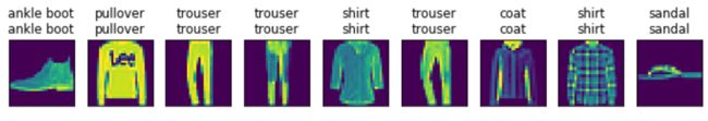
预测
import matplotlib.pyplot as plt
X, y = iter(test_iter).next()

def get_fashion_mnist_labels(labels):
    text_labels = ['t-shirt', 'trouser', 'pullover', 'dress', 'coat', 'sandal', 'shirt', 'sneaker', 'bag', 'ankle boot']
    return [text_labels[int(i)] for i in labels]

def show_fashion_mnist(images, labels):
    # 这⾥的_表示我们忽略(不使⽤)的变量
    _, figs = plt.subplots(1, len(images), figsize=(12, 12)) # 这里注意subplot 和subplots 的区别
    for f, img, lbl in zip(figs, images, labels):
        f.imshow(tf.reshape(img, shape=(28, 28)).numpy())
        f.set_title(lbl)
        f.axes.get_xaxis().set_visible(False)
        f.axes.get_yaxis().set_visible(False)
    plt.show()

true_labels = get_fashion_mnist_labels(y.numpy())
pred_labels = get_fashion_mnist_labels(tf.argmax(net(X), axis=1).numpy())
titles = [true + '\n' + pred for true, pred in zip(true_labels, pred_labels)]

show_fashion_mnist(X[0:9], titles[0:9])
softmax回归的简洁实现
import tensorflow as tf
from tensorflow import keras
获取和读取数据
fashion_mnist = keras.datasets.fashion_mnist
(x_train, y_train), (x_test, y_test) = fashion_mnist.load_data()
归一化
x_train = x_train / 255.0
x_test = x_test / 255.0
定义和初始化模型
model = keras.Sequential([
    keras.layers.Flatten(input_shape=(28, 28)),
    keras.layers.Dense(10, activation=tf.nn.softmax)
])
softmax和交叉熵损失函数
loss = 'sparse_categorical_crossentropy'
定义优化算法
optimizer = tf.keras.optimizers.SGD(0.1)
训练模型
model.compile(optimizer=tf.keras.optimizers.SGD(0.1),
              loss = 'sparse_categorical_crossentropy',
              metrics=['accuracy'])

model.fit(x_train,y_train,epochs=5,batch_size=256)
输出:
Train on 60000 samples
Epoch 1/5
60000/60000 [==============================] - 1s 20us/sample - loss: 0.7941 - accuracy: 0.7408
Epoch 2/5
60000/60000 [==============================] - 1s 11us/sample - loss: 0.5729 - accuracy: 0.8112
Epoch 3/5
60000/60000 [==============================] - 1s 11us/sample - loss: 0.5281 - accuracy: 0.8241
Epoch 4/5
60000/60000 [==============================] - 1s 11us/sample - loss: 0.5038 - accuracy: 0.8296
Epoch 5/5
60000/60000 [==============================] - 1s 11us/sample - loss: 0.4866 - accuracy: 0.8351
比较模型在测试数据集上的表现情况
test_loss, test_acc = model.evaluate(x_test, y_test)
print('Test Acc:',test_acc)
输出:
- 1s 55us/sample - loss: 0.4347 - accuracy: 0.8186
Test Acc: 0.8186
定义一个绘图函数xyplot。
%matplotlib inline
import tensorflow as tf
from matplotlib import pyplot as plt
import numpy as np
import random

def use_svg_display():
    # 用矢量图显示
    %config InlineBackend.figure_format = 'svg'

def set_figsize(figsize=(3.5, 2.5)):
    use_svg_display()
    # 设置图的尺寸
    plt.rcParams['figure.figsize'] = figsize

def xyplot(x_vals, y_vals, name):
    set_figsize(figsize=(5, 2.5))
    plt.plot(x_vals.numpy(), y_vals.numpy())
    plt.xlabel('x')
    plt.ylabel(name + '(x)')
relu
x = tf.Variable(tf.range(-8,8,0.1),dtype=tf.float32)
y = tf.nn.relu(x)
xyplot(x, y, 'relu')
绘制ReLU函数的导数
with tf.GradientTape() as t:
    t.watch(x)
    y=y = tf.nn.relu(x)
dy_dx = t.gradient(y, x)
xyplot(x, dy_dx, 'grad of relu')
sigmoid ( x ) = 1 1 + exp ( − x ) \operatorname{sigmoid}(x)=\frac{1}{1+\exp (-x)} sigmoid(x)=1+exp(−x)1
Sigmoid
y = tf.nn.sigmoid(x)
xyplot(x, y, 'sigmoid')
sigmoid ′ ( x ) = sigmoid ( x ) ( 1 − sigmoid ( x ) ) \operatorname{sigmoid}^{\prime}(x)=\operatorname{sigmoid}(x)(1-\operatorname{sigmoid}(x)) sigmoid′(x)=sigmoid(x)(1−sigmoid(x))
with tf.GradientTape() as t:
    t.watch(x)
    y=y = tf.nn.sigmoid(x)
dy_dx = t.gradient(y, x)
xyplot(x, dy_dx, 'grad of sigmoid')
tanh函数
tanh ( x ) = 1 − exp ( − 2 x ) 1 + exp ( − 2 x ) \tanh (x)=\frac{1-\exp (-2 x)}{1+\exp (-2 x)} tanh(x)=1+exp(−2x)1−exp(−2x)
y = tf.nn.tanh(x)
xyplot(x, y, 'tanh')
tanh ′ ( x ) = 1 − tanh 2 ( x ) \tanh ^{\prime}(x)=1-\tanh ^{2}(x) tanh′(x)=1−tanh2(x)
with tf.GradientTape() as t:
    t.watch(x)
    y=y = tf.nn.tanh(x)
dy_dx = t.gradient(y, x)
xyplot(x, dy_dx, 'grad of tanh')
多层感知机的从零开始实现
import tensorflow as tf
import numpy as np
import sys
sys.path.append("..") # 为了导入上层目录的d2lzh_tensorflow
import d2lzh_tensorflow2 as d2l
print(tf.__version__)
获取和读取数据
from tensorflow.keras.datasets import fashion_mnist
(x_train, y_train), (x_test, y_test) = fashion_mnist.load_data()
batch_size = 256
x_train = tf.cast(x_train, tf.float32)
x_test = tf.cast(x_test, tf.float32)
x_train = x_train/255.0
x_test = x_test/255.0
train_iter = tf.data.Dataset.from_tensor_slices((x_train, y_train)).batch(batch_size)
test_iter = tf.data.Dataset.from_tensor_slices((x_test, y_test)).batch(batch_size)
定义模型参数
num_inputs, num_outputs, num_hiddens = 784, 10, 256
W1 = tf.Variable(tf.random.normal(shape=(num_inputs, num_hiddens),mean=0, stddev=0.01, dtype=tf.float32))
b1 = tf.Variable(tf.zeros(num_hiddens, dtype=tf.float32))
W2 = tf.Variable(tf.random.normal(shape=(num_hiddens, num_outputs),mean=0, stddev=0.01, dtype=tf.float32))
b2 = tf.Variable(tf.random.normal([num_outputs], stddev=0.1))
定义激活函数
def relu(x):
    return tf.math.maximum(x,0)
定义模型
def net(X):
    X = tf.reshape(X, shape=[-1, num_inputs])
    h = relu(tf.matmul(X, W1) + b1)
    return tf.math.softmax(tf.matmul(h, W2) + b2)
定义损失函数
def loss(y_hat,y_true):
    return tf.losses.sparse_categorical_crossentropy(y_true,y_hat)
训练模型
我们直接调用d2l包中的train_ch3函数,它的实现已经在3.6节里介绍过。我们在这里设超参数迭代周期数为5,学习率为0.5
num_epochs, lr = 5, 0.5
params = [W1, b1, W2, b2]
d2l.train_ch3(net, train_iter, test_iter, loss, num_epochs, batch_size, params, lr)
输出:
epoch 1, loss 0.8208, train acc 0.693, test acc 0.804
epoch 2, loss 0.4784, train acc 0.822, test acc 0.832
epoch 3, loss 0.4192, train acc 0.843, test acc 0.850
epoch 4, loss 0.3874, train acc 0.857, test acc 0.858
epoch 5, loss 0.3651, train acc 0.864, test acc 0.860
多层感知机的简洁实现
import tensorflow as tf
from tensorflow import keras
fashion_mnist = keras.datasets.fashion_mnist
定义模型
model = tf.keras.models.Sequential([
    tf.keras.layers.Flatten(input_shape=(28, 28)),
    tf.keras.layers.Dense(256, activation='relu',),
    tf.keras.layers.Dense(10, activation='softmax')
])
读取数据并训练模型
fashion_mnist = keras.datasets.fashion_mnist
(x_train, y_train), (x_test, y_test) = fashion_mnist.load_data()
x_train = x_train / 255.0
x_test = x_test / 255.0
model.compile(optimizer=tf.keras.optimizers.SGD(lr=0.5),
             loss = 'sparse_categorical_crossentropy',
             metrics=['accuracy'])
model.fit(x_train, y_train, epochs=5,
              batch_size=256,
              validation_data=(x_test, y_test),
              validation_freq=1)
输出:
Train on 60000 samples, validate on 10000 samples
Epoch 1/5
60000/60000 [==============================] - 2s 33us/sample - loss: 0.7428 - accuracy: 0.7333 - val_loss: 0.5489 - val_accuracy: 0.8049
Epoch 2/5
60000/60000 [==============================] - 1s 22us/sample - loss: 0.4774 - accuracy: 0.8247 - val_loss: 0.4823 - val_accuracy: 0.8288
Epoch 3/5
60000/60000 [==============================] - 1s 21us/sample - loss: 0.4111 - accuracy: 0.8497 - val_loss: 0.4448 - val_accuracy: 0.8401
Epoch 4/5
60000/60000 [==============================] - 1s 21us/sample - loss: 0.3806 - accuracy: 0.8600 - val_loss: 0.5326 - val_accuracy: 0.8132
Epoch 5/5
60000/60000 [==============================] - 1s 21us/sample - loss: 0.3603 - accuracy: 0.8681 - val_loss: 0.4217 - val_accuracy: 0.8448
训练误差(training error)和泛化误差(generalization error)。
通俗来讲,前者指模型在训练数据集上表现出的误差,后者指模型在任意一个测试数据样本上表现出的误差的期望,并常常通过测试数据集上的误差来近似。
让我们以高考为例来直观地解释训练误差和泛化误差这两个概念。训练误差可以认为是做往年高考试题(训练题)时的错误率,泛化误差则可以通过真正参加高考(测试题)时的答题错误率来近似。
机器学习模型应关注降低泛化误差。
验证数据集(validation data set)
从严格意义上讲,测试集只能在所有超参数和模型参数选定后使用一次。不可以使用测试数据选择模型,如调参。由于无法从训练误差估计泛化误差,因此也不应只依赖训练数据选择模型。鉴于此,我们可以预留一部分在训练数据集和测试数据集以外的数据来进行模型选择。这部分数据被称为验证数据集,简称验证集(validation set)。例如,我们可以从给定的训练集中随机选取一小部分作为验证集,而将剩余部分作为真正的训练集。
K折交叉验证
由于验证数据集不参与模型训练,当训练数据不够用时,预留大量的验证数据显得太奢侈。一种改善的方法是K折交叉验证(K-fold cross-validation)。在K折交叉验证中,我们把原始训练数据集分割成K个不重合的子数据集,然后我们做K次模型训练和验证。每一次,我们使用一个子数据集验证模型,并使用其他K−1个子数据集来训练模型。在这K次训练和验证中,每次用来验证模型的子数据集都不同。最后,我们对这K次训练误差和验证误差分别求平均。
欠拟合和过拟合
接下来,我们将探究模型训练中经常出现的两类典型问题:
一类是模型无法得到较低的训练误差,我们将这一现象称作欠拟合(underfitting);
另一类是模型的训练误差远小于它在测试数据集上的误差,我们称该现象为过拟合(overfitting)。

在实践中,我们要尽可能同时应对欠拟合和过拟合。虽然有很多因素可能导致这两种拟合问题,在这里我们重点讨论两个因素:模型复杂度和训练数据集大小。
https://tangshusen.me/2018/12/09/vc-dimension/
多项式函数拟合实验
理解模型复杂度和训练数据集大小对欠拟合和过拟合的影响
import tensorflow as tf
import numpy as np
import matplotlib.pyplot as plt
%matplotlib inline
生成数据集
y = 1.2 x − 3.4 x 2 + 5.6 x 3 + 5 + ϵ y=1.2 x-3.4 x^{2}+5.6 x^{3}+5+\epsilon y=1.2x−3.4x2+5.6x3+5+ϵ
其中噪声项服从均值为0、标准差为0.1的正态分布。训练数据集和测试数据集的样本数都设为100。
n_train, n_test, true_w, true_b = 100, 100, [1.2, -3.4, 5.6], 5
features = tf.random.normal(shape=(n_train + n_test, 1))
poly_features = tf.concat([features, tf.pow(features, 2), tf.pow(features, 3)],1)
# x, x^2, x^3, 1
print(poly_features.shape)
labels = (true_w[0] * poly_features[:, 0] + true_w[1] * poly_features[:, 1]+ true_w[2] * poly_features[:, 2] + true_b)
print(tf.shape(labels))
labels += tf.random.normal(labels.shape,0,0.1)
看一看生成的数据集的前两个样本。
features[:2], poly_features[:2], labels[:2]

(,
 ,
 )
定义、训练和测试模型
定义作图函数semilogy,其中 y 轴使用了对数尺度。
# 本函数已保存在d2lzh_tensorflow2包中方便以后使用
from IPython import display
def use_svg_display():
    """Use svg format to display plot in jupyter"""
    display.set_matplotlib_formats('svg')

def set_figsize(figsize=(3.5, 2.5)):
    """Set matplotlib figure size."""
    use_svg_display()
    plt.rcParams['figure.figsize'] = figsize
def semilogy(x_vals, y_vals, x_label, y_label, x2_vals=None, y2_vals=None,
             legend=None, figsize=(3.5, 2.5)):
    set_figsize(figsize)
    plt.xlabel(x_label)
    plt.ylabel(y_label)
    plt.semilogy(x_vals, y_vals)
    if x2_vals and y2_vals:
        plt.semilogy(x2_vals, y2_vals, linestyle=':')
        plt.legend(legend)
    plt.show()
模型定义部分放在fit_and_plot函数中
num_epochs, loss = 100, tf.losses.MeanSquaredError()

def fit_and_plot(train_features, test_features, train_labels, test_labels):
    net = tf.keras.Sequential()
    net.add(tf.keras.layers.Dense(1))
    batch_size = min(10, train_labels.shape[0])
    train_iter = tf.data.Dataset.from_tensor_slices(
        (train_features, train_labels)).batch(batch_size)
    test_iter = tf.data.Dataset.from_tensor_slices(
        (test_features, test_labels)).batch(batch_size)
    optimizer = tf.keras.optimizers.SGD(learning_rate=0.01)
    train_ls, test_ls = [], []
    for _ in range(num_epochs):
        for X, y in train_iter:
            with tf.GradientTape() as tape:
                l = loss(y, net(X))

            grads = tape.gradient(l, net.trainable_variables)
            optimizer.apply_gradients(zip(grads, net.trainable_variables))

        train_ls.append(loss(train_labels, net(train_features)).numpy().mean())
        test_ls.append(loss(test_labels, net(test_features)).numpy().mean())
    print('final epoch: train loss', train_ls[-1], 'test loss', test_ls[-1])
    semilogy(range(1, num_epochs + 1), train_ls, 'epochs', 'loss',
             range(1, num_epochs + 1), test_ls, ['train', 'test'])
    print('weight:', net.get_weights()[0],
          '\nbias:', net.get_weights()[1])
三阶多项式函数拟合(正常):
fit_and_plot(poly_features[:n_train, :], poly_features[n_train:, :],
             labels[:n_train], labels[n_train:])

final epoch: train loss 0.0076061427 test loss 0.009977359
weight: [[ 1.1857017]
 [-3.3969326]
 [ 5.6001344]]
bias: [4.9984303]

线性函数拟合(欠拟合)
fit_and_plot(features[:n_train, :], features[n_train:, :], labels[:n_train],
             labels[n_train:])

final epoch: train loss 175.32323 test loss 394.3198
weight: [[18.400213]]
bias: [-1.3679209]

训练样本不足(过拟合)
fit_and_plot(poly_features[0:2, :], poly_features[n_train:, :], labels[0:2],
             labels[n_train:])

final epoch: train loss 0.14469022 test loss 201.26407
weight: [[2.843685  ]
 [0.80718964]
 [2.8566866 ]]
bias: [1.8927275]

高维线性回归实验
y = 0.05 + ∑ i = 1 p 0.01 x i + ϵ y=0.05+\sum_{i=1}^{p} 0.01 x_{i}+\epsilon y=0.05+i=1∑p0.01xi+ϵ
%matplotlib inline
import tensorflow as tf
from tensorflow.keras import layers, models, initializers, optimizers, regularizers
import numpy as np
import matplotlib.pyplot as plt
import d2lzh_tensorflow2 as d2l

n_train, n_test, num_inputs = 20, 100, 200
true_w, true_b = tf.ones((num_inputs, 1)) * 0.01, 0.05

features = tf.random.normal(shape=(n_train + n_test, num_inputs))
labels = tf.keras.backend.dot(features, true_w) + true_b
labels += tf.random.normal(mean=0.01, shape=labels.shape)
train_features, test_features = features[:n_train, :], features[n_train:, :]
train_labels, test_labels = labels[:n_train], labels[n_train:]
随机初始化模型参数的函数。该函数为每个参数都附上梯度。
def init_params():
    w = tf.Variable(tf.random.normal(mean=1, shape=(num_inputs, 1)))
    b = tf.Variable(tf.zeros(shape=(1,)))
    return [w, b]
定义L2范数惩罚项。这里只惩罚模型的权重参数。
def l2_penalty(w):
    return tf.reduce_sum((w**2)) / 2
定义训练和测试
batch_size, num_epochs, lr = 1, 100, 0.003
net, loss = d2l.linreg, d2l.squared_loss
optimizer = tf.keras.optimizers.SGD()
train_iter = tf.data.Dataset.from_tensor_slices(
    (train_features, train_labels)).batch(batch_size).shuffle(batch_size)

def fit_and_plot(lambd):
    w, b = init_params()
    train_ls, test_ls = [], []
    for _ in range(num_epochs):
        for X, y in train_iter:
            with tf.GradientTape(persistent=True) as tape:
                # 添加了L2范数惩罚项
                l = loss(net(X, w, b), y) + lambd * l2_penalty(w)
            grads = tape.gradient(l, [w, b])
            d2l.sgd([w, b], lr, batch_size, grads)
        train_ls.append(tf.reduce_mean(loss(net(train_features, w, b),
                             train_labels)).numpy())
        test_ls.append(tf.reduce_mean(loss(net(test_features, w, b),
                            test_labels)).numpy())
    d2l.semilogy(range(1, num_epochs + 1), train_ls, 'epochs', 'loss',
                 range(1, num_epochs + 1), test_ls, ['train', 'test'])
    print('L2 norm of w:', tf.norm(w).numpy())
当lambd设为0时,我们没有使用权重衰减。结果训练误差远小于测试集上的误差。这是典型的过拟合现象。
fit_and_plot(lambd=0)
使用权重衰减
fit_and_plot(lambd=3)
简洁实现
def fit_and_plot_tf2(wd, lr=1e-3):
    model = tf.keras.models.Sequential()
    model.add(tf.keras.layers.Dense(1,
                                 kernel_regularizer=regularizers.l2(wd),
                                    bias_regularizer=None))
    model.compile(optimizer=tf.keras.optimizers.SGD(lr=lr),
                 loss=tf.keras.losses.MeanSquaredError())
    history = model.fit(train_features, train_labels, epochs=100, batch_size=1,
              validation_data=(test_features, test_labels),
             validation_freq=1,verbose=0)
    train_ls = history.history['loss']
    test_ls = history.history['val_loss']
    dl2.semilogy(range(1, num_epochs + 1), train_ls, 'epochs', 'loss',
                     range(1, num_epochs + 1), test_ls, ['train', 'test'])
    print('L2 norm of w:', tf.norm(model.get_weights()[0]).numpy())
fit_and_plot_tf2(0, lr)
fit_and_plot_tf2(3, lr)
Tensorflow2函数接口说明
在聊GradientTape之前,我们不得不提一下自动微分技术,要知道在自动微分技术之前,机器学习社区中很少发挥这个利器,一般都是用Backpropagation(反向传播算法)进行梯度求解,然后使用SGD等进行优化更新。梯度下降法(Gradient Descendent)是机器学习的核心算法之一,自动微分则是梯度下降法的核心,梯度下降是通过计算参数与损失函数的梯度并在梯度的方向不断迭代求得极值。来自:
https://blog.csdn.net/DBC_121/article/details/108044938
GradientTape
GradientTape在模型中使用是,一般配合Optimizer使用,优化器有一个方法apply_gradients()用于优化梯度
tensorflow 提供tf.GradientTape api来实现自动求导功能。只要在tf.GradientTape()上下文中执行的操作,都会被记录与“tape”中,然后tensorflow使用反向自动微分来计算相关操作的梯度。可训练变量(由tf.Variable或创建tf.compat.v1.get_variable,trainable=True在两种情况下均为默认值)将被自动监视。通过watch在此上下文管理器上调用方法,可以手动监视张量。
例如,考虑函数y = x * x,x = 3.0时的梯度可以计算为:
import tensorflow as tf

x = tf.constant(3.0)
with tf.GradientTape() as tape:
	tape.watch(x)
	y = x * x
dy_dx = tape.gradient(y, x) # 求微分 tf.Tensor(6.0, shape=(), dtype=float32)
可以嵌套GradientTapes来计算高阶导数,如下
x = tf.constant(2.0)
with tf.GradientTape() as tape:
  tape.watch(x)
  with tf.GradientTape() as tt:
    tt.watch(x)
    y = x * x
  dy_dx = tt.gradient(y, x) # tf.Tensor(4.0, shape=(), dtype=float32)
dy2_dx2 = tape.gradient(dy_dx, x) # tf.Tensor(2.0, shape=(), dtype=float32)
默认情况下,GradientTape将自动监视在上下文中访问的所有可训练变量, 如果要对监视哪些变量进行精细控制,可以通过将watch_accessed_variables = False传递给tape构造函数来禁用自动跟踪:
with tf.GradientTape(watch_accessed_variables=False) as tape:
  tape.watch(variable_a)
  y = variable_a ** 2  # 梯度作用于`variable_a`.
  z = variable_b ** 3  # 由于`variable_b` 没有被watch,所有不会计算梯度
请注意,在使用模型时,应确保在使用watch_accessed_variables = False时变量存在,否则,这将导致你的迭代中没有使用梯度:
a = tf.keras.layers.Dense(32)
b = tf.keras.layers.Dense(32)

with tf.GradientTape(watch_accessed_variables=False) as tape:
  tape.watch(a.variables)  # 由于此时尚未调用`a.build`,因此`a.variables`将返回一个空列表,并且tape将不会监视任何内容。
  result = b(a(inputs))
  tape.gradient(result, a.variables)  # 该计算的结果将是“None”的列表,因为不会监视a的变量
reduce_sum()
reduce_sum() 是求和函数,在 tensorflow 里面,计算的都是 tensor,可以通过调整 axis =0,1 的维度来控制求和维度。
tf.norm():范数
reshape()
函数把行向量 x x x的形状改为(3, 4),也就是一个3行4列的矩阵,并记作 X X X。除了形状改变之外, X X X 中的元素保持不变。
X = tf.reshape(x,(3,4))
X
随机生成tensor中每个元素的值。下面我们创建一个形状为(3, 4)的tensor。它的每个元素都随机采样于均值为0、标准差为1的正态分布。
tf.random.normal(shape=[3,4], mean=0, stddev=1)
tf.cast()
执行 tensorflow 中张量数据类型转换,比如读入的图片如果是int8类型的,一般在要在训练前把图像的数据格式转换为float32。
cast定义:
cast(x, dtype, name=None)
第一个参数 x: 待转换的数据(张量)
第二个参数 dtype: 目标数据类型
第三个参数 name: 可选参数,定义操作的名称
tf.transpose(): 转置
tf.concat()
我们也可以将多个tensor连结(concatenate)。下面分别在行上(维度0,即形状中的最左边元素)和列上(维度1,即形状中左起第二个元素)连结两个矩阵。可以看到,输出的第一个tensor在维度0的长度( 6 )为两个输入矩阵在维度0的长度之和( 3+3 ),而输出的第二个tensor在维度1的长度( 8 )为两个输入矩阵在维度1的长度之和( 4+4 )。
tf.concat([X,Y],axis = 0), tf.concat([X,Y],axis = 1)
(,
 )
tf.Variable()
TensorFlow中tf.Variable的用法解析
https://blog.csdn.net/ding_programmer/article/details/95536343
矢量计算表达式
import tensorflow as tf
from time import time

a = tf.ones((1000,))
b = tf.ones((1000,))
向量相加的一种方法是,将这两个向量按元素逐一做标量加法。
start = time()
c = tf.Variable(tf.zeros((1000,)))
for i in range(1000):
    c[i].assign(a[i] + b[i])
time() - start
输出:
0.31618547439575195
向量相加的另一种方法是,将这两个向量直接做矢量加法。
start = time()
c.assign(a + b)
time() - start
Copy to clipboardErrorCopied
输出:
0.0
广播机制
a = tf.ones((3,))
b = 10
a+b
输出:
python中yield的用法详解——最简单,最清晰的解释
首先,如果你还没有对yield有个初步分认识,那么你先把yield看做“return”,这个是直观的,它首先是个return,普通的return是什么意思,就是在程序中返回某个值,返回之后程序就不再往下运行了。看做return之后再把它看做一个是生成器(generator)的一部分(带yield的函数才是真正的迭代器),好了,如果你对这些不明白的话,那先把yield看做return,然后直接看下面的程序,你就会明白yield的全部意思了
https://blog.csdn.net/mieleizhi0522/article/details/82142856/
tf.gather(params,indices,axis=0 )
从params的axis维根据indices的参数值获取切片
tf.assign()
tf.assign(ref, value, validate_shape=True, use_locking=None, name=None)
释义:将 value 赋值给 ref,即 ref = value
ref,变量
value,值
tf.assign_add(ref, value, use_locking=None, name=None)
释义:将值 value 加到变量 ref 上, 即 ref = ref + value
ref,变量
value,值
tf.assign_sub(ref, value, use_locking=None, name=None)
释义:变量 ref 减去 value值,即 ref = ref - value
ref,变量
value,值