数据可视化

import numpy as np
import pandas as pd
import matplotlib.pyplot as plt

plt.rcParams['font.sans-serif'] = 'SimHei'
plt.rcParams['axes.unicode_minus'] = False

%config InlineBackend.figure_format = 'svg'

import warnings

warnings.filterwarnings('ignore')

数据可视化

1.1 Matplotlib

画图给内部人员看，主要用于数据探索，核心组件包括：

• 画布：figure() —> 绘图的基础
• 坐标系：subplot() —> 一个画布上可以有多个坐标系
• 坐标轴：plot() / scatter() / bar() / pie() / hist() / boxplot()
  • 趋势: 折线图(plot)
  • 关系：散点图(scatter)
  • 差异：柱状图(bar)
  • 占比：饼图(pie)
  • 分布：直方图(hist)
  • 描述统计信息：箱线图（盒须图）(boxplot)

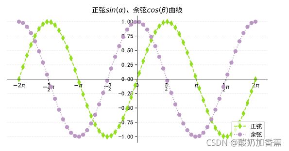
折线图（plot）

x = np.linspace(-2 * np.pi, 2 * np.pi, 60)
y1 = np.sin(x)
y2 = np.cos(x)

np.random.rand(3) # 可以用作三原色

# 创建画布
plt.figure(figsize=(8, 4), dpi=120)
# 创建坐标系
ax = plt.subplot(1, 1, 1)
ax.spines['top'].set_visible(False)
ax.spines['right'].set_visible(False)
ax.spines['left'].set_position('center')
ax.spines['bottom'].set_position('center')
# 绘图
plt.plot(x, y1, color=np.random.rand(3), marker='d', linestyle='--')
plt.plot(x, y2, color=np.random.rand(3), marker='o', linestyle=':')
# 定制横轴的刻度
plt.xticks(
    np.arange(-2 * np.pi, 2 * np.pi + 1, 0.5 * np.pi),
    labels=[r'$-2\pi$', r'$-\frac{3}{2}\pi$', r'$-\pi$', r'$-\frac{\pi}{2}$',
            '0', r'$\frac{\pi}{2}$', r'$\pi$', r'$\frac{3}{2}\pi$', r'$2\pi$']
)
# 定制横轴和纵轴
# plt.xlabel('横轴')
# plt.ylabel('纵轴')
# 定制标题和纵轴的标签
plt.title(r'正弦$sin(\alpha)$、余弦$cos(\beta)$曲线')
# 定制图例
plt.legend(loc='lower right', labels=['正弦', '余弦'])
# 定制网格线
plt.grid(axis='y', alpha=0.25, linestyle='--')
plt.show()

plt.get_cmap('RdYlBu')

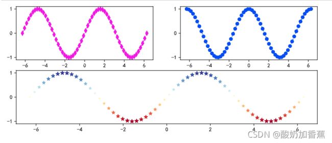
散点图（scatter）

# 在一个画布上创建多个坐标系
plt.figure(figsize=(10, 4), dpi=120)
plt.subplot(2, 2, 1)
# 绘制折线图
plt.plot(x, y1, color=np.random.rand(3), marker='d', linestyle='--', label='余弦')
plt.subplot(2, 2, 2)
plt.plot(x, y2, color=np.random.rand(3), marker='o', linestyle=':', label='余弦')
plt.subplot(2, 1, 2)
# 绘制散点图
plt.scatter(x, y1, c=y1 * 50, cmap='RdYlBu', marker='*', s=np.abs(y1 * 50) + 5, label='正弦')
plt.show()

动图

# 动图
import gif
import IPython.display as disp

@gif.frame
def draw(xi):
    plt.subplots(1, figsize=(10, 4), dpi=120)
    plt.plot(xi, np.sin(xi), marker='x', color='r', linestyle='--')
    plt.xlim([-7, 7])
    plt.xticks(np.arange(-2 * np.pi, 2 * np.pi + 1, 0.5 * np.pi))
    plt.ylim([-1, 1])


frames = []
x = np.linspace(-2 * np.pi, 2 * np.pi, 120)
for i in range(x.size // 4):
    frame = draw(x[:(i + 1) * 4])
    frames.append(frame)
gif.save(frames, 'a.gif', duration=0.2, unit='s')
disp.HTML('')

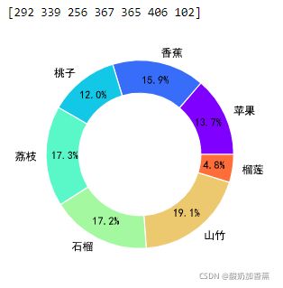
饼图（pie）

from matplotlib import cm

# 饼图
plt.figure(figsize=(4, 4), dpi=120)
data = np.random.randint(100, 500, 7)
print(data)
labels = ['苹果', '香蕉', '桃子', '荔枝', '石榴', '山竹', '榴莲']
plt.pie(
    data,
    # 自动显示百分比
    autopct='%.1f%%',
    # 饼图的半径
    radius=1,
    # 修改饼的颜色
    colors=cm.rainbow(np.arange(data.size) / data.size),
    # 百分比文字到圆心的距离
    pctdistance=0.8,
    # 分离距离
    # explode=[0.1, 0, 0.05, 0, 0, 0, 0],
    # 显示阴影
    # shadow=True,
    # 字体属性
    textprops=dict(fontsize=10, color='black'),
    # 楔子属性
    wedgeprops=dict(linewidth=1, width=0.35, edgecolor='white'),
    # 每一块饼的标签
    labels=labels
)
plt.show()

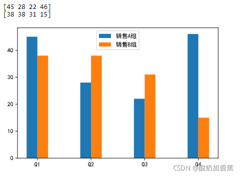
柱状图（bar）

# 堆叠柱状图
labels = np.arange(4)
group1 = np.random.randint(20, 50, 4)
print(group1)
group2 = np.random.randint(10, 60, 4)
print(group2)
plt.bar(labels - 0.1, group1, 0.2, label='销售A组')
# 通过bottom属性设置数据堆叠
plt.bar(labels + 0.1, group2, 0.2, label='销售B组')
plt.xticks(np.arange(4), labels=['Q1', 'Q2', 'Q3', 'Q4'])
plt.legend()
plt.show()

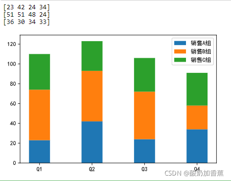
# 堆叠柱状图
labels = np.array(['Q1', 'Q2', 'Q3', 'Q4'])
group1 = np.random.randint(20, 50, 4)
print(group1)
group2 = np.random.randint(10, 60, 4)
print(group2)
group3 = np.random.randint(30, 40, 4)
print(group3)
plt.bar(labels, group1, 0.4, label='销售A组')
# 通过bottom属性设置数据堆叠
plt.bar(labels, group2, 0.4, bottom=group1, label='销售B组')
plt.bar(labels, group3, 0.4, bottom=group1 + group2, label='销售C组')
plt.legend()
plt.show()

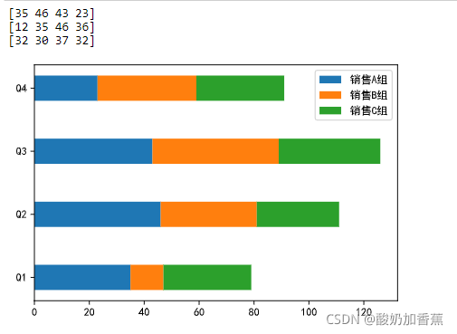
# 水平柱状图
# 堆叠柱状图
labels = np.array(['Q1', 'Q2', 'Q3', 'Q4'])
group1 = np.random.randint(20, 50, 4)
print(group1)
group2 = np.random.randint(10, 60, 4)
print(group2)
group3 = np.random.randint(30, 40, 4)
print(group3)
plt.barh(labels, group1, 0.4, label='销售A组')
# 通过bottom属性设置数据堆叠
plt.barh(labels, group2, 0.4, left=group1, label='销售B组')
plt.barh(labels, group3, 0.4, left=group1 + group2, label='销售C组')
plt.legend()
plt.show()

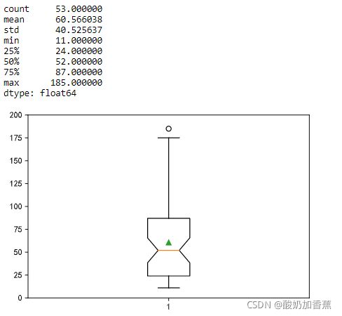
箱线图（boxplot）

# 箱线图
data = np.random.randint(10, 100, 50)
data = np.append(data, 185)
data = np.append(data, 175)
data = np.append(data, 155)
print(pd.Series(data).describe())
plt.boxplot(data, whis=1.5, showmeans=True, notch=True)
plt.ylim([0, 200])
plt.show()

面积图（stackplot）

# 面积图
plt.figure(figsize=(6, 3))
days = np.arange(7)
sleeping = [7, 8, 6, 6, 7, 8, 10]
eating = [2, 3, 2, 1, 2, 3, 2]
working = [7, 8, 7, 8, 6, 2, 3]
playing = [8, 5, 9, 9, 9, 11, 9]
plt.stackplot(days, sleeping, eating, working, playing)
plt.legend(['睡觉', '吃饭', '工作', '玩耍'], fontsize=10)
plt.show()

雷达图

# 雷达图（极坐标折线图）
labels = np.array(['速度', '力量', '经验', '防守', '发球', '技术'])
malong_values = np.array([93, 95, 98, 92, 96, 97])
shuigu_values = np.array([30, 40, 65, 80, 45, 60])
angles = np.linspace(0, 2 * np.pi, labels.size, endpoint=False)
# 加一条数据让图形闭合
malong_values = np.concatenate((malong_values, [malong_values[0]]))
shuigu_values = np.concatenate((shuigu_values, [shuigu_values[0]]))
angles = np.concatenate((angles, [angles[0]]))
# 创建画布
plt.figure(figsize=(4, 4), dpi=120)
# 创建坐标系
ax = plt.subplot(projection='polar')
# 绘图和填充
plt.plot(angles, malong_values, color='r', marker='o', linestyle='--', linewidth=2)
plt.fill(angles, malong_values, color='r', alpha=0.3)
plt.plot(angles, shuigu_values, color='g', marker='o', linestyle='--', linewidth=2)
plt.fill(angles, shuigu_values, color='g', alpha=0.2)
# 设置文字和网格线
ax.set_thetagrids(angles[:-1] * 180 / np.pi, labels, fontsize=10)
ax.set_rgrids([0, 20, 40, 60, 80, 100], fontsize=10)
ax.legend(['马龙', '水谷隼'])
plt.show()

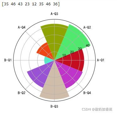
玫瑰图（圆形柱状图）

# 玫瑰图（圆形柱状图）
x = np.array([f'A-Q{i}' for i in range(1, 5)] + [f'B-Q{i}' for i in range(1, 5)])
y = np.array(group1.tolist() + group2.tolist())
print(y)
theta = np.linspace(0, 2 * np.pi, x.size, endpoint=False)
width = 2 * np.pi / x.size
colors = np.random.rand(8, 3)
# 将柱状图投影到极坐标
ax = plt.subplot(projection='polar')
plt.bar(theta, y, width=width, color=colors, bottom=0)
ax.set_thetagrids(theta * 180 / np.pi, x, fontsize=10)
plt.show()

3D柱状图

# 3D柱状图
plt.figure(figsize=(8, 4), dpi=120)
ax = plt.subplot(projection='3d')

colors = ['r', 'g', 'b']
yticks = range(2020, 2017, -1)
for idx, y in enumerate(yticks):
    x_data = [f'{x}季度' for x in '一二三四']
    z_data = np.random.randint(100, 600, 4)
    ax.bar(x_data, z_data, zs=y, zdir='y', color=colors[idx], alpha=0.5)
ax.set_xlabel('季度')
ax.set_ylabel('年份')
ax.set_zlabel('销量')
ax.set_yticks(yticks)
plt.show()

词云图

!pip install jieba

import re
import jieba

with open('data/test.txt', encoding='utf-8') as file:
    content = file.read()
content = re.sub(r'\s', '', content)

words = jieba.lcut(content)
len(words)

def get_stopwords(file):
    with open(file, 'r', encoding='utf-8') as file:
        stopword_list = [word.strip('\n') for word in file.readlines()]
    return stopword_list


stop_words1 = get_stopwords('data/哈工大停用词表.txt')
stop_words2 = get_stopwords('data/中文停用词库.txt')
# 将两组停词合并到一个集合中（集合判断元素是否存在更快）
stop_words = set(stop_words1 + stop_words2)
len(stop_words)

# 从分词的结果中去掉没有实际意义的停词
words = [word for word in words if word not in stop_words]
print(len(words))

pip install wordcloud

# 绘制词云图
from wordcloud import WordCloud
from PIL import Image

txt = ' '.join(words)
mask = np.array(Image.open('images/china_map.jpg'))
wc = WordCloud(
    font_path='fonts/SimHei.ttf',
    mask=mask,
    width=1200,
    height=800,
    background_color='white',
    max_words=100,
)
wc.generate(txt)
wc.to_file('result.png')

1.2 seaborn

import seaborn as sns

# tips = sns.load_dataset('tips')
tips = pd.read_csv('data/tips.csv')
tips.head()

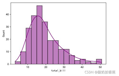
sns.histplot(tips['total_bill'], bins=16, color="purple", kde=True)
plt.show()

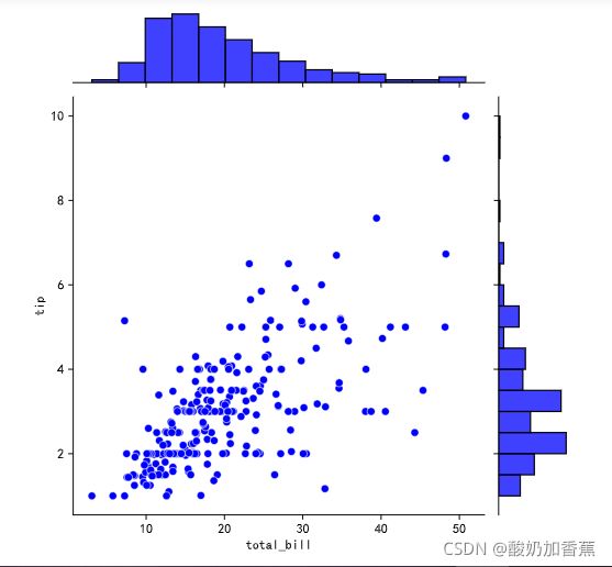
sns.jointplot(x='total_bill', y='tip', data=tips, color='blue')
plt.show()

sns.jointplot(x='total_bill', y='tip', data=tips, color='blue', kind='hex')
plt.show()

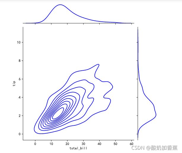
sns.jointplot(x='total_bill', y='tip', data=tips, color='blue', kind='kde')
plt.show()

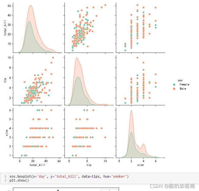
sns.pairplot(tips, hue='sex', palette="Set2")
plt.show()

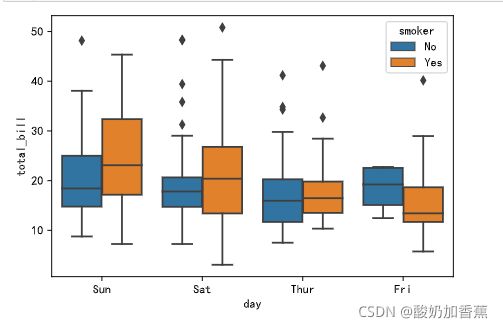
sns.boxplot(x='day', y='total_bill', data=tips, hue='smoker')
plt.show()

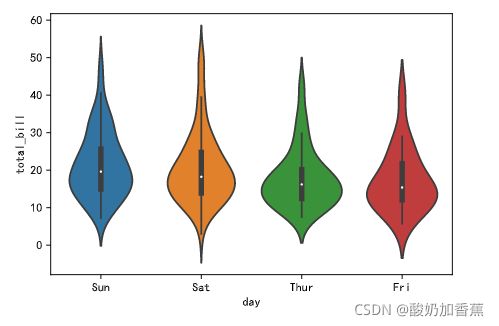
sns.violinplot(x='day', y='total_bill', data=tips)
plt.show()

sns.set_palette('rainbow')
sns.color_palette()