CBIR: Indexing and Retrieval--基于内容的图像检索：索引和检索

CBIR: Indexing and Retrieval

• Shape Feature Extraction
  • Boundary-based Representation of Shape
  • Region-based Representation of Shape
  • Spatial Relationships of Objects
  • MPEG-7 Visual Shape Descriptors
    • 3D Shape Descriptor - Shape Spectrum
    • Region-Based Shape Descriptor - ART
    • Contour-Based Shape Descriptor
    • 2D/3D Shape Descriptor
• Multidimensional Feature Indexing
  • Similarity Between Features
  • Similarity-based Search
  • Dimensionality Reduction
• Semantic representation for image retrieval
• References

Shape Feature Extraction

The use of object shape is one of the most challenging problems in creating efficient CBIR. The object's shape plays a critical role in searching for similar image objects (e.g. texts or trademarks in binary images or specific boundaries of target objects in aerial or space images, etc.). In image retrieval, one expects that the shape description is invariant to scaling, rotation, and translation of the object and is naturally either 2D or 3D depending on the object.

Shape features are less developed than their colour and texture counterparts because of the inherent complexity of representing shapes. In particular, image regions occupied by an object have to be found in order to describe its shape, and a number of known segmentation techniques combine the detection of low-level colour and texture features with region-growing or split-and-merge processes. But generally it is hardly possible to precisely segment an image into meaningful regions using low-level features due to the variety of possible projections of a 3D object into 2D shapes, the complexity of each individual object shape, the presence of shadows, occlusions, non-uniform illumination, varying surface reflectivity, and so on (Castelli & Bergman, 2002).

After segmenting objects, their shapes have to be described, indexed, and compared. However no mathematical description is able to fully capture all aspects of visually perceived shapes as well as shape comparison is also a very difficult problem. The elusive nature of shape hinders any formal analysis of a trade-off between the complexity of shape description and its ability to describe and compare shapes of interest. At present CBIR exploits two large groups of 2D shape descriptors, namely, contour-based and region-based, representing either an outer boundary (or contour) or an entire region. These representations can also be combined together.

Both boundary-based and region-based descriptions are perceptually meaningful and interchangeable in the sense that each one can be used as a basis to compute the other (e.g. by filling-in the interior region or by tracing the boundary). But the explicit shape features available in each type of description are quite different, so that an ideal description should include both boundaries and regions in order to obtain more efficient retrieval.

Boundary-based Representation of Shape

Boundary representation describes the closed curve surrounding the shape. The curve can be specified in numerous ways, e.g., by chain codes, polygons, circular arcs, splines, or boundary Fourier descriptors: 

The boundary features such as an ordered polygonal approximation allow for a user query formulated as a sketch. Generally, the sketch is deformed to adjust to the shape of target models, and the amount of deformation, e.g. the energy for an elastic deformation model. Such a  deformable template  represents shape variability by allowable transformations of a template.

Let, for example, the 1D boundary template be modelled, by a second-order spline parametrised by arc length. The template deforms to match a sketch in an "elastic" way, by maximising the edge strength integral along the curve while minimising the strain and bending energies modelled by integrals of the first and second derivatives of the deformation along the curve. Shape similarity is measured by combining the strain and bending energy, edge strength along the curve, and curve complexity (Castelli & Bergman, 2002).

Curvature of planar curves is one of the most powerful tools for representing and interpreting objects in an image. Although curvature extraction from a digitized object contour would seem to be a rather simple task, few methods exist that are at the same time easy to implement, fast, and reliable in the presence of noise. (Leymarie & Levine). Important features of an object's boundary related to the curvature function are extrema or peaks of curvature, points of inflection (i.e., zero-crossings of curvature), and segments of constant curvature that correspond to straight line segments or circular arcs of the boundary.

Let c(t) = (x(t), y(t)) and c(x, y) = 0 present an explicit (with two Cartesian parametric equations) and implicit definitions of the same planar curve, respectively. The curvature k in each point of the curve measures the curve's bending, i.e. the speed of changing of the angle between the tangent vector to the curve and the x-axis. Let s and φ denote the arc length along the curve and the tangential angle, respectively. It is shown in differential geometry that: 

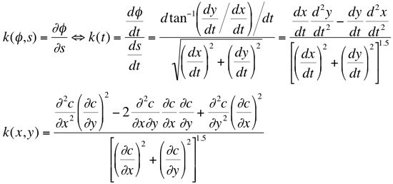
Typically, curvature of a discrete curve is computed from orientation of successive digital curve segments using either filtering and differentiation methods or difference of slope estimates ( Leymarie & Levine ). The former approximate local curvature by convolving a discrete orientation representation of a contour with a smoothing and differentiation filter, usually, the derivative of a Gaussian of variable size. Alternatively, the orientation data is differentiated by computing the first difference of the angle formed by nearby points and then smoothed with a Gaussian filter to remove noise. This yields a multiscale representation if a set of different sized filters is used, but usually has a lower signal-to-noise ratio because the direct differentiation of discrete orientation data amplifies noise. The second group of methods estimates curvature at each point by taking the angular difference between slopes (orientation) of two line segments fitted to the data before and after each point. This can be repeated for line segments of varying length. The extent of data smoothing is governed in both methods by the filer or line size. The latter methods give good results in the presence of boundary noise but require more computations due to fitting straight lines to the nerighbouring data at each contour pixel.

Region-based Representation of Shape

Region-based, or interior descriptions of shape specify the object's "body" within the closed boundary. Such a shape is represented with moment invariants, or a collection of primitives such as rectangles, disks, quadrics, etc., deformable templates, skeletons, or simply a set of points.

A skeleton represents each shape with the axis of symmetry between a pair of boundaries. The simplest skeleton is given by the medial axis defined as the trace of a locus of inscribed maximum-size circles. The skeleton is usually represented by a graph.

A shock set created by propagation from boundaries (similar to a "grassfire" initiated from the boundaries) is another variant of the medial axis. Shocks are singularities formed from the collisions of propagating fronts. By adding shock dynamics to each point and grouping the monotonically flowing shocks into branches, a shock graph is formed. Comparing to the skeletal one, the shock graph results in a finer partition of the medial axis.

Because shape is also defined in terms of presence and distribution of oriented parts, the quantitative characteristics of objects' orientation within an image, for instance, angular spectra of image components or edge directionality, may serve as global shape descriptors. In particular, the blobworld model efficiently describes objects separated from the background by replacing each object with a "blob", or an ellipse identified by the centroid and the scatter matrix. The blob is characterised also with the mean texture and the two dominant colours. The initial images are segmented using an Expectation - Maximisation (EM) algorithm based on colour and texture features.

Spatial Relationships of Objects

Shape features include also spatial relationships of objects, in particular, topological and directional relationships. The first group describes the relations between object boundaries, such as "near to", "within", or "adjacent to". The second group shows the relative positions of objects with respect to each other, e.g. "in front of", "on the left of", or "on top of". Such spatial relationships are frequently described with theattributed-relational graph (ARG). Nodes of the graph represent objects, and an arc between two nodes represents a certain relationship between them.

MPEG-7 Visual Shape Descriptors

That shape often carries semantic information follows from the fact that many characteristic objects can be visually recognised solely from their shapes. This distinguishes shape from other elementary visual features such as colour, motion, or texture. The latter are equally important, but do not identify an object (Bober, 2001; Sikora, 2001). But the notion of object shape has many meanings. To deal with 3D real-world objects, MPEG-7 standard has a 3D shape descriptor. The use of only 2D projections of 3D objects onto an image plane lead to notions of region- and contour-based similarity outlined below: 

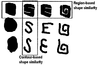
MPEG-7 supports both botions of similarity using region-based and contour-based shape descriptors. When a 3D object model is unknown but a set of 2D views specifies jointly the 3D properties of the object, MPEG-=7 provides a 2D/3D shape descriptor. Because the reconstruction of the original shape from the description is not required, the MPEG-7 descriptors are very compact. Also they are invariant to scaling, rotation, translation, and to some shape distortions due to imaging conditions (e.g. a perspective transformation under changing angle of view), non-rigid object deformations, or distortions resulting from image segmentation or shape extraction processes.

3D Shape Descriptor - Shape Spectrum

The MPEG-7  3D shape detector  exploits the shape spectrum concept extending to 3D meshes the shape index used for a loing time as a local 3D shape measure. The shape index SI _Σ  of an orientable 3D surface Σ, at point  p , is defined as ( Duncan & Olson, 1993 ): 

where  k ₁ ( p ) and  k ₁ ( p );  k ₁ ( p ) ≥  k ₂ ( p ), are the principal curvatures at point  p . The shape index indicates the local convexity of a 3D surface and is undefined for planar regions where both the principal curvatures are equal to zero.

The principal curvatures are the eigenvalues of the local Hessian matrix H(p) at point p. Provided that z = Σ(x,y) is a 3D surface over the coordinate (x,y)-plane, the Hessian at point p = (x,y,z) is the symmetric 2×2 matrix of second derivatives: 

Both its determinant and the trace (sum of the diagonal elements) are invariant to orientation of ( x,y )-coordinate frame. The first eigenvector (such that corresponds to the maximum eigenvalue  k ₁ ( p )) is the direction of the maximum curvature, i.e. of the largest second directional derivative, and the second eigenvector (with the minimum eigenvalue  k ₂ ( p )) is the direction of the smallest curvature.

Shape spectrum is the histogram of the shape index values over the entire 3D surface. For 3D meshes, the shape index is computed for each vertex of the mesh. The spectrum is invariant to scaling, rotation, and translation. The default descriptor has histogram with 100 bins, 12 bit per bin. The descriptor has two additional variables: (i) the relative area of planar surface regions in the mesh, with respect to the entire area of the 3D mesh, and (ii) the relative area of all polygonal components where the shape index cannot be reliably estimated with respect to the entire area of the 3D mesh.

Region-Based Shape Descriptor - ART

The region-based shape descriptor uses region moments which are invariant to transformations as the shape feature. It can describe complex objects with multiple disconnected regions as well as simple objects with or without holes (Bober, 2001; Sikora, 2001), gives a compact description of multiple disjoint regions simultaneously, allows for splitting of an object during segmentation into disconnected sub-regions, providing the information which regions it was split into is retained, and is robust to segmentation noise (e.g. salt-and-pepper noise).

The descriptor uses a complex-valued Angular Radial Transformation (ART) defined on a unit disk in polar coordinates with a set of ART basis functions V_mn(ρ, θ) of order n and m that are separable along the angular and radial directions: 

The shape of a greyscale image  g (ρ, θ) in polar coordinates is represented by a set of ART coefficients  f_nm : 

The default region-based shape descriptor uses 35 coefficients quantised to 4 bits per coefficient. Examples below show shapes that can be efficiently described by the region-based descriptor (e.g. fish images in set (B) would be identified as mutually similar but dissimilar to the ones in the four other sets): 

(A)	(B)	(C)	(D)	(E)

Contour-Based Shape Descriptor

The contour-based shape descriptor is based on the curvature scale-space (CSS) representation of the contour (Mokhtarian & Mackworth, 1992 If an object contains several disjoint regions, each region has a separate contour-based shape description. A CSS index for matching shapes indicates the height of the most prominent peak and the horizontal and vertical positions of the remaining peaks in a specific CSS "image" describing a contour shape. The descriptor includes the eccentricity and circularity values of the original and filtered contours (6 bits each), the number of peaks in the CSS image (6 bits), the height of the highest peak (7 bits), and the x and y positions of the remaining peaks (9 bits per peak). The average size of the descriptor is 112 bits per contour

This descriptor is efficient for describing objects for which characteristic shape features are contained in the contour (e.g. the shapes in set A below) or objects having similar region but very different contour properties (the set B below); 

(A)	(B)
(C)	(D)	(E)

The descriptor has been selected on the basis of comprehensive comparative tests performed by the MPEG team. These tests have shown that the CSS outperforms most popular other approaches, including Fourier-based shape description techniques, shape representations based on Zernike moments or turning angles, and wavelet-based techniques

To form a CSS description of a contour, N equi-distant points {(x_i,y_i): i = 1, ..., N} are selected on the contour, starting from an arbitrary point 1 on the contour and following the contour clockwise. The contour is gradually smoothed by repetitive application of a low-pass moving filter (0.25, 0.50, 0.25) to two series X = {x₁, x₁, ..., x_N} and X = {x₁, x₁, ..., x_N} of the individual x and y coordinates of the selected Ncontour points. During the smoothing, the contour evolves. Its concavities are gradually flatten-out until the contour becomes convex (see also the SQUID retrieval system developed under supervision of Prof. J. Kittler and Dr. F. Mokhtarian which uses the CSS shape representation and shape-based queries).

The contour evolution can be illustrated using a special CSS "image" associated with the evolutionary process (it need not be explicitly formed but is convenient to demonstrate the CSS representation). Horizontal coordinates x_css of the CSS image correspond to the N indices of the selected contour points that represent the contour. Vertical coordinates y_css of the CSS image correspond to the number of iterations of smoothing applied to the coordinate sets X and Y: 

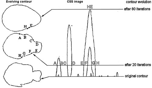
Horizontal line in the CSS image with the vertical coordinate  y _css  relates to the smoothed contour obtained after  y _css  passes of the filter. For each smoothed contour, the zero-crossings of its curvature function that separate concave and convex parts of the contour are marked on the corresponding horizontal line at the locations indicating the positions of these zero-crossings along the contour. The CSS image has characteristic (prominent) peaks, and their coordinates ( x _css ,  y _css ) are ordered by decreasing values  y _css , non-linearly transformed, and quantisede to form the descriptor. In the above example, the shape evolution during filtering (left) produces the corresponding CSS image (right). The contour curvature zero crossings and the corresponding points in the CSS image are marked A, B, ..., H.

2D/3D Shape Descriptor

The shape of a 3D object can be approximately represented with a limited number of 2D shapes taken from different viewing directions. The 2D/3D shape descriptor forms a complete 3D view-based representation of the object by combining 2D descriptors representing its visible 3D shape seen from different view angles. Generally, any 2D visual descriptor, e.g. contour shape, region shape, colour, or texture, can be used. The 2D/3D descriptor allows for integrating the 2D descriptors used in the image plane to describe features of real-world 3D objects. Then a similarity matching between 3D objects is based on matching multiple corresponding pairs of 2D views of the objects.

Multidimensional Feature Indexing

Content-based visual information retrieval (CBIR) is based on extracting and indexing of metadata, objects and features, and relations between objects in images and video. Indexing pursues the goals to accelerate the queries and overcome the "curse of dimensionality" in performing the content-based search. Metadata indexing is a complex application-dependent problem that includes automatic analysis of unstructured text descriptions, definition of image standards and translation between different standards. But indexing of objects and features in multimedia databases is even more complex and difficult problem that has no general solution. For instance, descriptions of spatial relations in images are mostly developed in very special application domains such as modern geographic information systems (GIS).

Feature-level image representation reduces the QBE (query by image example) retrieval to computation of similarity between multidimensional feature vectors describing either a whole image or a portion of it. In the first case (whole image match) the query template is an entire image and the similar images have to be retrieved. A single feature vector is used for indexing and retrieval. Such matching was used in retrieving photographic images and adopted in early CBIR systems like QBIC.

In the second case (subimage match) the query template is a portion of an image, and the retrieval results in images with similar portions or just in portions of images containing desired objects. Such a partial matching is important for many application areas such as remotely sensed images of the Earth or medical images. Most today's CBIR systems support subimage retrieval by segmenting the stored images and associating a feature vector with each potentially interesting segment. The segmentation may be data-independent (a set of non-overlapping or overlapping rectangular regions called blocks or windows) or data-dependent (adaptive).

Similarity Between Features

Today's CBIR involves different low-level colour, texture, and shape descriptors. Typically these descriptors are represented by multidimensional vectors, and similarity between two images is specified by some quantitative measure in the feature space. For the vector feature space, a range query results in retrieving all the points lying within a hyperrectangle aligned with the coordinate axes. But to support nearest-neighbour andwithin-distance (or A-cut) queries, the feature space must possess a metric or a dissimilarity measure. The same vector metrics can be used to define the dissimilarity between statistical distributions, although these latter have also specific dissimilarity measures. Most common dissimilarity / similarity measures are as follows:

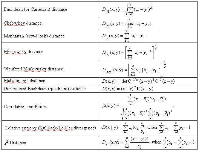
Dissimilarity / similarity between two n-dimensional vectors x and y 
(the n×n matrix C is a covariance matrix for a data set; 
the matrix K is a positive definite but not necessarily a covariance matrix; 
the bars denote average values of the vector components for the entire the data set; 
vector components in the relative entropy or chi-square distance are positive.

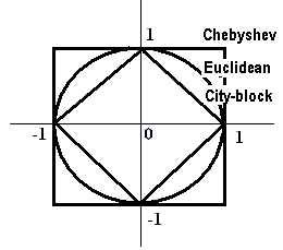
The unit sphere under the Euclidean distance is a conventional spherical ball. Under the Chebyshev distance, a unit ball is a hypersquare aligned with the coordinate axes and inscribing the unit Euclidean sphere. A ball under the city-block distance is also a hypersquare, having vertices on the coordinate axes and inscribed in the Euclidean ball. For the Minkowsky distance with  p  > 2, a unit ball looks like a "fat sphere" lying between the Euclidean and Chebyshev balls, and with 1 <  p  < 2 it is a "slender sphere" between the city-block and Euclidean balls.

The unit spheres under Chebyshev, Euclidean, and city-block distance.

The Chebyshev, Euclidean, and city-block distances are particular cases of the Minkowsky family of distances. All the Minkowsky distances differ in the way they combine the contributions of coordinate-wise differences d_i = x_i - y_i between the vectors x and y. When p = 1, all the absolute differences contribute equally to the distance D_[1](x,y). When p grows, the value D_[p](x,y) is increasingly determined by the maximum of the absolute differences,whereas the overall contribution of all the other differences becomes less and less significant.

Similarity-based Search

A brute-force sequential scanning of the database is computationally infeasible. To search in large databases, indexing of the vectors and search keys that accelerates the retrieval becomes a must. Most popular indexing structures are based on representing the feature vectors as points in a multidimensional vector space and accounting for either particular regions in it (vector space indexes), or pairwise distances between the objects in a database (metric space indexes). From the algorithmic viewpoint, the indexing structures are nonhierachical, recursive, and projection based(Castelli & Bergman, 2002). Nonhierachical indexing divides the feature space into regions such that each region a query point belongs to is found in a fixed number of steps. Recursive indexing organised the space as a tree in order to optimise computational efficiency of the retrieval. Projection-based indexing tries to search on the linear or nonlinear projections of database points onto a subspace in the feature space. This latter method relates closely to reduction of dimensionality of the feature space for a given database.

Nonhierarchical indexing maps the n-dimensional vectors onto the real line using a space-filling curve (e.g., Peano or Hilbert one). The mapped records are indexed with a 1D indexing structure. Because space-filling curves preserve to some extent the neighbourhood relations between initial vectors, range queries, nearest-neighbour queries, and A-cut queries are approximated rather closely along the linear mapping.

Recursive indexing divides recursively the search space into successively smaller regions that depend on the data set being indexed. The resulting decomposition of the space is well-represented by a tree. The most popular trees in recursive indexing are quad-trees, k-n-trees and R-trees. Quad-trees in the n-dimensional space are trees of degree 2ⁿ, so that each nonterminal node has 2ⁿ children. Each nonterminal node of a n-quad-tree divides the n-dimensional space into 2ⁿ hyperrectangles aligned with the coordinate axes. The partitioning is obtained by simultaneously splitting each coordinate axis into two parts. K-n-trees divide the space with (n-1)-dimensional hyperplanes perpendicular to a specific coordinate axis selected as a function of the data related to the node. Each nonterminal node has at least two children.

R-trees generalise multiway B-trees allowing, with a scalar search key, an extremely efficient search. For multidimensional indexing, the R-tree and its modifications are the best (Castelli & Bergman, 2002). The R-tree is a B-tree-like indexing structure where each internal node represents a k-dimensional hyperrectangle rather than a scalar range. The hyperrectangle of the node contains all the hyperrectangles of the children. The rectangles can overlap, so that more than one subtree under a node may have to be visited during a search. To improve a performance, the R^*-tree is proposed that minimises the overlap among the nodes.

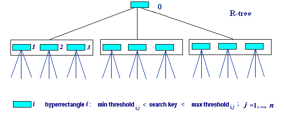
Multiway search R-tree: a vector search key is compared to the hyperrectangles in each successive node.

But both R-trees and R^*-trees work well until the dimension of the indexing key is less than 20. Otherwise dimension reduction should be performed before indexing the feature vectors. The main problem is that our three-dimensional geometric intuition fails when the number of dimensions grows, e.g., almost all the volume of a 100-dimensional hypercube is outside the largest inscribed sphere:

Ratio between the volumes of the minimum bounding hypercube and the hypersphere

Therefore, hypercubes are extremely poor approximations of hyperspheres although most of the indexing structures partition the space into hypercubes or hyperrectangles. As a result, R-trees become extremely inefficient for performing an  A -cut query with the Euclidean distance because the R-tree search transforms that query into the range one defined by the minimum bounding hyperrectangle.

Another difficulty caused by the "curse of dimensionality" is that the high-dimensional vector spaces demonstrate no tightly concentrated clusters of data items typical to the low-dimensional cases. Let us consider a simple example: n-dimensional feature vectors x=[x₁, ..., x_n] with independent components having each the standard normal (Gaussian) distribution with zero mean and the standard deviation s. The Euclidean distanced between the two independent vectors x and y of that type is defined as follows

d ² = ( x ₁ -  y ₁) ² + ... + ( x _n -  y _n) ²

Therefore, the mathematical expectation and the variance of the square distance are 2ns² and 4ns⁴, respectively. If s = 1, then in the one-dimensional (1D) case with n = 1, the square distance between the two features is distributed asymmetrically around the value 2 with the standard deviation equal to 2 so that a vast majority of the distances d are within the range [0, 2.8]. But in the 100-dimensional case (n = 100) the distribution is almost symmetrical around 200 with the approximate standard deviation 20. Thus most of the distances d are within the range [11.4, 16.1], and there are no points "close" to or "far" from the query. It is evident that in the multi-dimensional case the nearest-neighbour or within-distance (A-cut) queries become essentially meaningless.

Fortunately, in practice the feature space has often a local structure that makes the notion of close neighbourhood of a query image still meaningful. Also, the features are usually interdependent and can be well-approximated by their projections onto an appropriate lower-dimensional space, where the distance- or similarity-based indexing behaves well. The mapping from a higher-dimensional to a lower-dimensional space is calleddimensionality reduction and performed by selecting a subset of variables (possibly after a linear transformation of the feature space), or multidimensional scaling, or geometric hashing (Castelli & Bergman, 2002).

Dimensionality reduction

Selection of a subset of variables reduces the dimensionality of the feature space by discarding "less characteristic" dimensions. These methods are popular in applied statistics and pursue the goal of minimising the error of approximation of the original vectors with lower-dimensional projections after a linear transformation of the feature space. The transformation makes the transformed features uncorrelated, that is, the covariance matrix of the transformed data set becomes diagonal. This method is known under different names, for instance, the Karhunen-Loeve transform (KLT), principal component analysis (PCA), or singular value decomposition (SVD). Although particular numerical algorithms may differ, all the above methods are equivalent in essence. The choice of variables is governed by the scatter (variance) of the data set around each new coordinate axis, the chosen subset of variables having usually to preserve a given percentage (e.g., 95% or 99%) of the total scatter of the original data set. This approach minimises the mean squared error of discarding each particular number of dimensions with smaller variance, so that the original vectors are closer in Euclidean distance to their decorrelated projections than with any other linear transformation. But the approach is data-dependent, computationally expensive, and suited well for only static databases. Dynamic databases with regularly inserted and deleted items need special (and usually computationally very expensive) techniques for effectively updating the KLT/PCA/SVD of a data set.

Principal component analysis (PCA) performs linear transformation of a number of possibly correlated feature vectors into a possibly smaller number of uncorrelated vectors called principal components. The first principal component accounts for the maximal variability in the feature vectors projected onto this line, and each next component accounts for the maximal remaining variability in the feature space. Let f_k; k = 1, ...,K, denote given n-dimensional vectors with the empirical mean m and the empirical covariance matrix S: 

The components  S_ij  of the covariance matrix estimate the covariances between the vector components  f_i  and  f_j , and the matrix component  S_ii  is the variance of the vector component  f_i . The symmetric matrix  S  has an orthogonal basis of the eigenvectors  e _i : 

The eigenvalues compared to the total sum of eigenvalues specify how much of the feature variability is concentrated along each particular eigenvector. The eigenvectors ordered by the desreasing eigenvalues λ _i , starting from the largest λ ₁ , form the orthogonal basis such that the first eigenvector is directed along the line of the largest variance of the feature vectors projected on it in the feature vector space; the second eigenvector has the direction of the line corresponding to the largest remaining variance, and so forth. Instead of using all the eigenvectors of the covariance matrix, the feature vectors can be approximated with only a few basis vectors of the orthogonal basis. If the feature vectors are actually concentrated in a linear subspace of dimension ν ≤  n , the PCA allows for reducing the data dimesionality from  n  to ν with no information loss and thus simplify the representation. Generally, the use of the ν eigenvectors with the largest eigenvalues and replacement of the initial feature  n -dimensional vectors with their ν-dimensional projections onto the linear subspace specified by the selected basis, give the minimum information losses in the mean-square sense: 

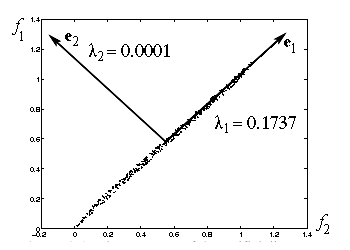
An example below (from  http://www.cis.hut.fi/jhollmen/dippa/node30.html ) shows the eigenvectors and eigenvalues for a set of the artificial 2D ( n  = 2) feature vectors  f  = ( f ₁ ,  f ₂ ) depicted with small dots. The calculated mean vector and covariance matrix result in the two eigenvectors drawn by arrows. The first eigenvalue λ ₁  = 0.1737 is much greater than the second eigenvalue λ ₂  = 0.0001. Therefore, the first eigenvector is responsible for almost all the feature variation, and this data set can be closely approximated with a 1D representation obtained by linear mapping (projection) of the feature vectors onto the line directed along the first eigenvector. 

Multidimensional scaling is based on nonlinear mapping of the n-dimensional feature space into m-dimensional one (m < n). There is no general theory or precise definition of this approach. In many cases the metric multidimensial scaling tries to minimise changes of the pairwise Euclidean distances between the objects in a data set, but numerous other statements of the problem exist. In general, nonlinear mapping can provide better dimensionality reduction than linear methods, but at the expense of much heavier computations. The approach is also data-dependent and poorly suited for dynamic databases.

Geometric hashing performs data-independent mapping of the n-dimensional feature space into a very low-dimensional one, namely, the 1D real line or the 2D real plane. Ideally, hashing spreads the database uniformly across the range of the low-dimensional space, so that the metric properties of the hashed space differ significantly from those of the original feature space. This is why geometric hashing is applied to indexing of low-dimensional feature spaces in the case when only their local metric properties need to be maintained. Also, the difficulties in designing a good hashing function grow with the dimensionality of the original space.

Generally, dimensionality reduction facilitates efficient indexing of multidimensional feature spaces, but the search is now performed on the transformed rather than original data. But in many cases the approximation reduces impacts of the "curse of dimensionality" and improves the retrieval. If only a particular class of queries has to be supported, more efficient multidimensional indexing structures can be developed. In particular, to capture the local structure of a database without involving computationally expensive multidimensional scaling, CSVD (Clustering with Singular Value Decomposition), proposed by Thomasian, Castelli, and Li, first partitions the data into homogeneous clusters and then separately reduces the dimensionality of each cluster. The number of the clusters is selected empirically, and the index is represented as a tree, each node containing the cluster parameters (the centroid and radius) and the dimensionality reduction information (the projection matrix and the number of retained dimensions). Nonleaf nodes contain information for assigning a query vector to its cluster and pointers to the children, each of which represents a separate cluster. Terminal nodes (leaves) contain an indexing scheme supporting nearest-neighbour queries.

Semantic representation for image retrieval

Meaningful analysis and retrieval of multimedia content depend on semantic representation, but how to describe multimedia content with semantic labels remains a challenging problem ( Wang & Manjunath ). It is very difficult to manually annotate images and videos as well as retrieve raw data. Thus automated semantic analysis is a must for efficient search and retrieval. The main problem in semantic labelling is a wide variation in visual apperance within objects of the same class. It becomes very time consuming and expensive to collect and formalise knowledge about each such class, and different classes may need specific types of labelling. An alternative approach is to build a statistical learning system that starts with a minimal knowledge and simple descriptors. Users then train the system via formative feedback before it can work with large databases.

References

• M. Bober. MPEG-7 visual shape descriptors. IEEE Transactions on Circuits and Systems for Video Technology, vol. 11, no. 6, 2001, 716 - 719.
•  V. Castelli and L. D. Bergman (Eds.). Image Databases: Search and Retrieval of Digital Imagery. Wiley: New York, 2002.
• B. S. Duncan and A. J. Olson. Shape analysis of molecular surfaces. Biopolymers, vol. 33, 1993, 231 - 238.
• A.Hanjalic, G. C. Langelaar, P. M. B. van Roosmalen, J. Biemond, and R. Lagendijk. Image and Video Data Bases: Restoration, Watermarking and Retrieval. Elsevier Science: Amsterdam, 2000.
• F. Leymarie and M. D. Levine. Curvature Morphology. Center for Intelligent Machines. TR-CIM-88-26. McGill University, Montreal, Canada. December 1988. 36p.
• J. M. Martinez, Ed. MPEG-7 Overview. ISO/IEC JTC1/SC29/WG11 No. 6828 (2004). On-line. http://www.chiariglione.org/mpeg/standards/mpeg-7/mpeg-7.htm#E12E27
• F. Mokhtarian and A. K. Mackworth. A theory of multiscale, curvature-based shape representation for planar curves. IEEE Transactions on Pattern Analysis and Machine Intelligence, vol. 14, 1992, 789 - 805.
•  S. M. Rahman (Ed.). Interactive Multimedia Systems. IRM Press: Hershey, 2002.
• T. K. Shih. Distributed Multimedia Databases: Techniques & Applications. Idea Group Publishing: Hershey, 2002.
• T. Sikora. The MPEG-7 visual standard for content description - an overview. IEEE Transactions on Circuits and Systems for Video Technology, vol. 11, no. 6, 2001, 696 - 702.
• A. W. M. Smeulders and R. Jain (Eds.). Image Databases and Multimedia Search. World Scientific: Singapore, 1997.
• L. Wang and B. S. Manjunath. A semantic representation for image retrieval. Proc. Int. Conf. on Image Processing (ICIP 2003), September 14 - 17, 2002, Barselona, Spain. IEEE CS Press: Los Alamitos, vol. 2, 2002, 523 - 526.

Return to the local table of contents

Return to the general table of contents

from: https://www.cs.auckland.ac.nz/courses/compsci708s1c/lectures/Glect-html/topic5c708FSC.htm