lstm自动编码器进行时间序列异常检测

人工智能与异常检测(Artificial Intelligence and Anomaly Detection)

Anomaly provides evidence that actual results differ from predicted results based on ML models. We are talking about price prediction and how ML model is behaving compared to actual price data. Here anomaly is defined as a point in time where the behavior of the system is unusual and significantly different from past behavior. So, going by this definition, an anomaly does not necessarily imply a problem. An important use case is the ability to detect anomalies by analyzing and learning the time series. That means AI can be used to detect anomalous data points in the time series by understanding the trends and changes seen from historical data.

一个nomaly提供的证据表明实际结果基于ML模型所预测的结果不同。 我们正在谈论价格预测以及与实际价格数据相比ML模型的行为方式。 在这里，异常被定义为系统行为异常且与过去行为显着不同的时间点。 因此，按照这个定义，异常并不一定意味着有问题。 一个重要的用例是能够通过分析和学习时间序列来检测异常。 这意味着，通过了解历史数据的趋势和变化，可以将AI用于检测时间序列中的异常数据点。

Much of the worlds data is streaming, time-series data, where anomalies give significant information in critical situations. However, detecting anomalies in streaming data is challenging, requiring to process data in real-time, and learn while simultaneously making predictions. The underlying system is often non-stationary, and detectors must continuously learn and adapt to changing statistics while simultaneously making predictions.

世界上许多数据都是按时间顺序排列的流数据，在紧急情况下异常会提供大量信息。 但是，检测流数据中的异常是一项挑战，需要实时处理数据，并在进行预测的同时进行学习。 底层系统通常是不稳定的，检测器必须不断学习并适应变化的统计信息，同时进行预测。

Here we will look at neural network (LSTM) implementations for use cases using time series data as examples. We will develop an anomaly detection model for Time Series data.

在这里，我们将以时间序列数据为例，研究用例的神经网络(LSTM)实现。 我们将为时间序列数据开发异常检测模型。

Let us load Henry Hub Spot Price data from EIA.

让我们从EIA加载Henry Hub现货价格数据。

print("....Data loading...."); print()
print('\033[4mHenry Hub Natural Gas Spot Price, Daily (Dollars per Million Btu)\033[0m')
def retrieve_time_series(api, series_ID):
  series_search = api.data_by_series(series=series_ID)
  spot_price = DataFrame(series_search)
  return spot_pricedef main():
  try:
    api_key = "....API KEY..."
    api = eia.API(api_key)
    series_ID = 'xxxxxx'
    spot_price = retrieve_time_series(api, series_ID)
    print(type(spot_price))
    return spot_price;
  except Exception as e:
    print("error", e)
    return DataFrame(columns=None)
spot_price = main()
spot_price = spot_price.rename({'Henry Hub Natural Gas Spot Price, Daily (Dollars per Million Btu)': 'price'}, axis = 'columns')
spot_price = spot_price.reset_index()
spot_price['index'] = pd.to_datetime(spot_price['index'].str[:-3], format='%Y %m%d')
spot_price['Date']= pd.to_datetime(spot_price['index'])
spot_price.set_index('Date', inplace=True) 
spot_price = spot_price.loc['2000-01-01':,['price']] 
spot_price = spot_price.astype(float)
print(spot_price)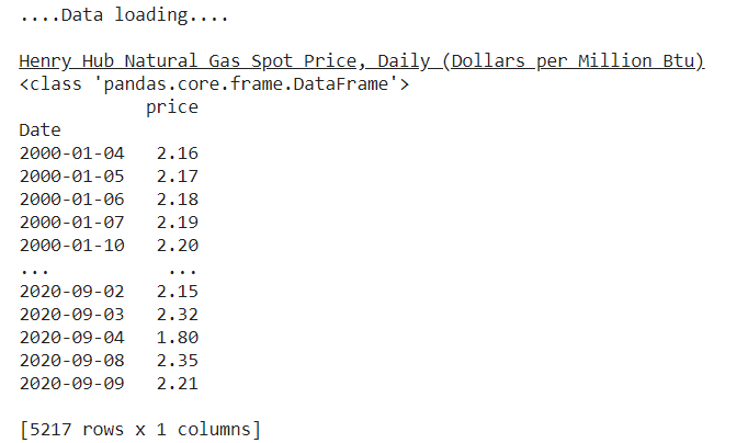

原始数据可视化 (Raw data visualization)

print('Historical Spot price visualization:')
plt.figure(figsize = (15,5))
plt.plot(spot_price)
plt.title('Henry Hub Spot Price (Daily frequency)')
plt.xlabel ('Date_time')
plt.ylabel ('Price ($/Mbtu)')
plt.show()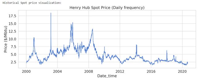

print('Missing values:', spot_price.isnull().sum()) 
# checking missing values
spot_price = spot_price.dropna() 
# dropping missing valies
print('....Dropped Missing value row....')
print('Rechecking Missing values:', spot_price.isnull().sum()) 
# checking missing values

The common characteristic of different types of market manipulation for data scientists would be the unexpected pattern/behavior in data.

对于数据科学家而言，不同类型的市场操纵的共同特征是数据的意外模式/行为。

# Generate a Boxplot
print('Box plot visualization:')
spot_price.plot(kind='box', figsize = (10,4))
plt.show()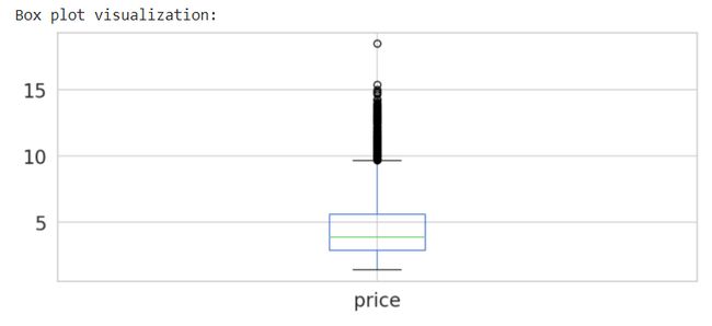

# Generate a Histogram plot
print('Histogram visualization:')
spot_price.plot(kind='hist', figsize = (10,4) )
plt.show()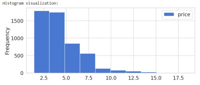

检测异常子序列 (Detecting anomalous subsequence)

Here, the goal is identifying an anomalous subsequence within a given long time series (sequence).

在此，目标是识别给定的长时间序列(序列)内的异常子序列。

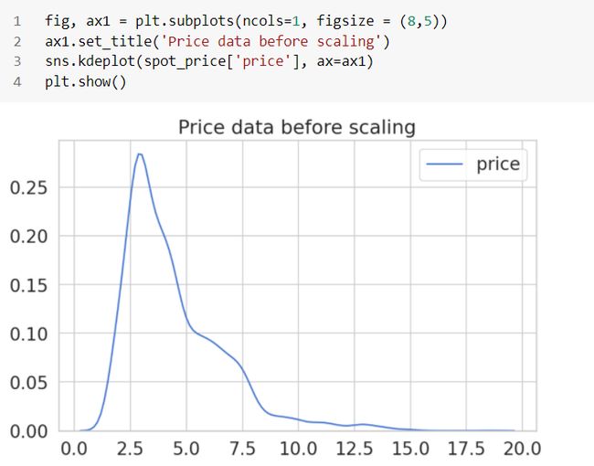
前处理 (Pre-processing)

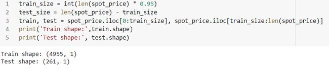
We’ll use 95% of the data and train our model on it:

我们将使用95％的数据并对模型进行训练：

Next, we’ll re-scale the data using the training data and apply the same transformation to the test data:

接下来，我们将使用训练数据重新缩放数据，并将相同的转换应用于测试数据：

robust = RobustScaler(quantile_range=(25, 75)).fit(train[['price']])
train['price'] = robust.transform(train[['price']])
test['price'] = robust.transform(test[['price']])

Finally, we’ll split the data into sub-sequences with the help of a helper function.

最后，我们将在辅助函数的帮助下将数据划分为子序列。

# helper function
def create_dataset(X, y, time_steps=1):
  a, b = [], []
  for i in range(len(X) - time_steps):
     v = X.iloc[i:(i + time_steps)].values
     a.append(v)
     b.append(y.iloc[i + time_steps])
  return np.array(a), np.array(b)# We’ll create sequences with 30 days of historical datan_steps = 30# reshape to 3D [n_samples, n_steps, n_features]X_train, y_train = create_dataset(train[['price']], train['price'], n_steps)
X_test, y_test = create_dataset(test[['price']], test['price'], n_steps)
print('X_train shape:', X_train.shape)
print('X_test shape:', X_test.shape)

Keras中的LSTM自动编码器 (LSTM Autoencoder in Keras)

Our Autoencoder should take a sequence as input and outputs a sequence of the same shape.We have a total of 5219 data points in the sequence and our goal is to find anomalies. We are trying to find out when data points are abnormal. If we can predict a data point at time t based on the historical data until t-1, then we have a way of looking at an expected value compared to an actual value to see if we are within the expected range of values for time t.

我们的自动编码器应将一个序列作为输入并输出相同形状的序列。我们在序列中共有5219个数据点，我们的目标是发现异常。 我们正在尝试找出数据点何时异常。 如果我们可以根据直到t-1的历史数据预测时间t的数据点，那么我们可以通过查看期望值与实际值的比较来查看我们是否在时间t的期望值范围内。

We can compare y_pred with the actual value (y_test). The difference between y_pred and y_test gives the error, and when we get the errors of all the points in the sequence, we end up with a distribution of just errors. To accomplish this, we will use a sequential model using Keras. The model consists of a LSTM layer and a dense layer. The LSTM layer takes as input the time series data and learns how to learn the values with respect to time. The next layer is the dense layer (fully connected layer). The dense layer takes as input the output from the LSTM layer, and transforms it into a fully connected manner. Then, we apply a sigmoid activation on the dense layer so that the final output is between 0 and 1.

我们可以将y_pred与实际值(y_test)进行比较。 y_pred和y_test之间的差异给出了错误，当我们获得序列中所有点的错误时，最终得到的只是错误的分布。 为此，我们将使用Keras的顺序模型。 该模型由LSTM层和致密层组成。 LSTM层将时间序列数据作为输入，并学习如何学习有关时间的值。 下一层是致密层(完全连接的层)。 密集层将LSTM层的输出作为输入，并将其转换为完全连接的方式。 然后，在密集层上应用S型激活，以使最终输出在0到1之间。

We also use the adam optimizer and the mean squared error as the loss function.

我们还使用亚当优化器和均方误差作为损失函数。

序列问题 (Issue with Sequences)

This is challenging because ML algorithms, and neural networks are designed to work with fixed length inputs. Another challenge with sequence data is that the temporal ordering of the observations can make it challenging to extract features suitable for use as input to supervised learning models

这是具有挑战性的，因为ML算法和神经网络被设计用于固定长度的输入。 序列数据的另一个挑战是，观测值的时间顺序可能使提取适合用作监督学习模型输入的特征具有挑战性

units = 64
dropout = 0.20
optimizer = 'adam'
loss = 'mae'
epochs = 20model = keras.Sequential()
model.add(keras.layers.LSTM(units=units, input_shape =(X_train.shape[1], X_train.shape[2])))
model.add(keras.layers.Dropout(rate=dropout))
model.add(keras.layers.RepeatVector(n=X_train.shape[1])) 
# RepeatVector layer repeats the input n times.
model.add(keras.layers.LSTM(units=units, return_sequences=True)) 
# Adding return_sequences=True in LSTM layer makes it return the sequence.
model.add(keras.layers.Dropout(rate=dropout))
model.add(keras.layers.TimeDistributed(keras.layers.Dense(units= X_train.shape[2])))
# TimeDistributed layer creates a vector with a length of the number of outputs from the previous layer.
model.compile(loss= loss, optimizer=optimizer)
history = model.fit(X_train, y_train, epochs=epochs, batch_size=32, validation_split=0.1, shuffle=False)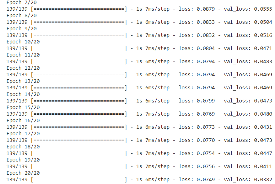

# history for loss
plt.figure(figsize = (10,5))
plt.plot(history.history['loss'])
plt.plot(history.history['val_loss'])
plt.title('model loss')
plt.ylabel('loss')
plt.xlabel('epoch')
plt.legend(['train', 'test'], loc='upper left')
plt.show()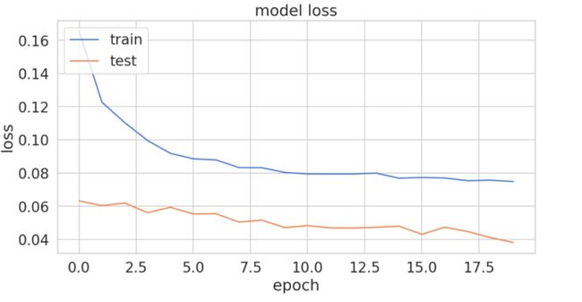

评价 (Evaluation)

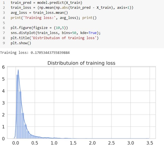
Once the model is trained, we can predict using test data set and compute the error (mae). Let’s start with calculating the Mean Absolute Error (MAE) on the training data.

训练模型后，我们可以使用测试数据集进行预测并计算误差(mae)。 让我们开始计算训练数据的平均绝对误差(MAE)。

MAE火车数据 (MAE on train data)

测试数据的准确性指标(Accuracy metrics on test data)

# MAE on the test data:
y_pred = model.predict(X_test)
print('Predict shape:', y_pred.shape); print();
mae = np.mean(np.abs(y_pred - X_test), axis=1)
# reshaping prediction
pred = y_pred.reshape((y_pred.shape[0] * y_pred.shape[1]), y_pred.shape[2])
print('Prediction:', pred.shape); print();
print('Test data shape:', X_test.shape); print();
# reshaping test data
X_test = X_test.reshape((X_test.shape[0] * X_test.shape[1]), X_test.shape[2])
print('Test data:', X_test.shape); print();
# error computation
errors = X_test - pred
print('Error:', errors.shape); print();
# rmse on test data
RMSE = math.sqrt(mean_squared_error(X_test, pred_reshape))
print('Test RMSE: %.3f' % RMSE);

RMSE is 0.099, which is low, and this is also evident from the low loss from the training phase after 20 epochs: loss: 0.0749— val_loss: 0.0382.

RMSE为0.099，这很低，这也可以从20个时期后训练阶段的低损失中看出：损失：0.0749- val_loss：0.0382。

阈值计算 (Threshold computation)

dist = np.linalg.norm(X_test - pred, axis=1);"""Sorting the scores/diffs and using a 0.80 as cutoff value to pick the threshold"""scores = dist.copy();
print('Score:', scores.shape);
scores.sort();
cut_off = int(0.80 * len(scores));
print('Cutoff value:', cut_off);
threshold = scores[cut_off];
print('Threshold value:', threshold);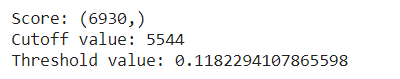

Objective is that, anomaly will be detected when the error is larger than selected threshold value.

目的是当误差大于选定的阈值时，将检测到异常。

score = DataFrame(index=test[n_steps:].index);
score['loss'] = mae; score['threshold'] = THRESHOLD;
score['anomaly'] = score['loss'] > score['threshold'];
score['price'] = test[n_steps:].price;
plt.figure(figsize = (10,5));
plt.plot(score.index, score['loss'], label='loss');
plt.plot(score.index, score['threshold'], label='threshold');
plt.xticks(rotation=90); plt.legend();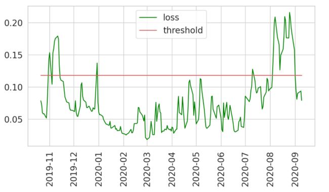

Looks like we’re thresholding extreme values quite well. Let’s create a DataFrame using only those:

看起来我们对极限值的要求很好。 让我们仅使用以下内容创建一个DataFrame：

异常报告格式 (Anomalies report format)

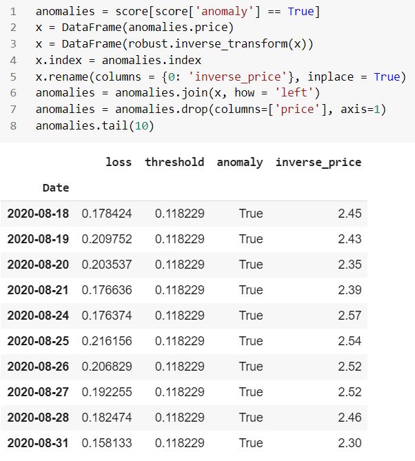
反向测试数据(Inverse test data)

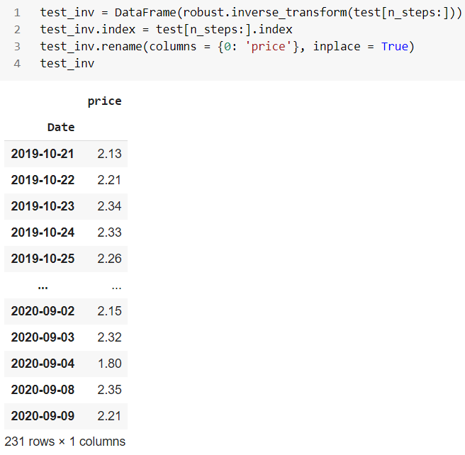
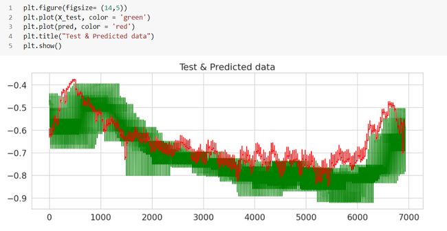
Finally, let’s look at the anomalies found in the testing data:

最后，让我们看一下测试数据中发现的异常：

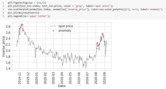
The red dots are the anomalies here and are covering most of the points with abrupt changes to the existing spot price. The threshold values can be changed as per the parameters we choose, especially the cutoff value. If we play around with some of the parameters we used, such as number of time steps, threshold cutoffs, epochs of the neural network, batch size, hidden layer etc., we can expect a different set of results.

红点是这里的异常，覆盖了大多数点，并且现有现货价格发生了突然变化。 阈值可以根据我们选择的参数进行更改，尤其是截止值。 如果我们使用一些我们使用的参数，例如时间步数，阈值截止，神经网络的历元，批处理大小，隐藏层等，我们可以期望得到一组不同的结果。

Here we have show a brief overview of finding anomalies in time series with respect to stock trading.

在这里，我们简要概述了如何发现与股票交易有关的时间序列异常。

结论 (Conclusion)

The main challenge related to anomaly detection is unknown nature of the anomaly. Therefore, it is impossible to use classical machine learning techniques to train the model, as we don’t have labels of time series with anomaly. One of the best machine learning methods is autoencoder based anomaly detection.

与异常检测相关的主要挑战是异常的未知性质。 因此，不可能使用经典的机器学习技术来训练模型，因为我们没有带有异常的时间序列标签。 最好的机器学习方法之一是基于自动编码器的异常检测。

Anomalies are crucial because they represent serious but exceptional events, and they can stimulate severe actions to be taken in a broad range of application regions. Though the stock market is highly efficient, it is impossible to prevent historical and long term anomalies. Therefore, the investors may use them to their advantage. Exploiting the anomalies to earn superior returns is a risk since the anomalies may or may not persist in the future.

异常非常重要，因为它们代表严重但异常的事件，并且它们可以刺激在广泛的应用区域中采取严厉的措施。 尽管股票市场非常高效，但无法防止历史和长期异常。 因此，投资者可以利用他们的优势。 利用异常情况获得较高的回报是一种风险，因为异常情况将来可能会或可能不会持续。

Connect me here.

在这里连接我。

Note: The programs described here are experimental and should be used with caution for any commercial purpose. All such use at your own risk….by Author…

注意：此处描述的程序是实验性的，出于商业目的应谨慎使用。 所有此类使用的风险均由您自己承担……作者作者…

翻译自: https://medium.com/swlh/time-series-anomaly-detection-with-lstm-autoencoders-7bac1305e713