Python银行风控模型的建立（解决Grapviz的中文显示问题）

Python银行风控模型的建立

一、用神经网络Sequential（序贯模型）搭建

1、背景：

700个数据，前8列作为x，最后一列为y，建立银行风控模型。（数据量不大）

二分类问题，损失函数用’binary_crossentropy’，指标也用metrics=[BinaryAccuracy()]

训练集和测试集8-2开，但我最后还是用y和yp比较模型精度，所以不应该要求精度太高（避免过拟合）

2、经过多次调参，最好的model代码如下

model = Sequential()

model.add(Dense(input_dim=8,units=800,activation='relu'))
model.add(Dropout(0.5))
model.add(Dense(input_dim=800,units=400,activation='relu'))
model.add(Dropout(0.5))
model.add(Dense(input_dim=400,units=1,activation='sigmoid'))

model.compile(loss='binary_crossentropy', optimizer='adam',metrics=[BinaryAccuracy()])
model.fit(x_train,y_train,epochs=1000,batch_size=128)

3、对比分析：

1、3层和4层的激活函数的效果基本一样，但是四层更耗时。

2、训练500次和1000次，精度下降，运行时间也减少；训练1000次比训练100次的精确度高0.1左右，运行时间大大缩短，从44s到6s；

3、relu激活函数比softsign激活函数更优，但是也较为耗时。

4、input_dim和units，传入数和批数小，精确度和损失值都会降下来，运行时间也会减少。

4、我的结论：

在数据量不大的情况下，综合考虑运行时间、精度、损失值，我认为，0.81左右的精度足够了，六秒运行时间还在接受范围内。

5、代码如下：

import pandas as pd
import numpy as np
#导入划分数据集函数
from sklearn.model_selection import train_test_split
#读取数据
datafile = 'C:/Users/86188/Desktop/Python数据挖掘与数据分析/My work/data2/bankloan2.xls'#文件路径
data = pd.read_excel(datafile)
x = data.iloc[:,:8]
y = data.iloc[:,8]
#划分数据集
x_train, x_test, y_train, y_test = train_test_split(x, y, test_size=0.2, random_state=100)
#导入模型和函数
from keras.models import Sequential
from keras.layers import Dense,Dropout
#导入指标
from keras.metrics import BinaryAccuracy
#导入时间库计时
import time
start_time = time.time()
#-------------------------------------------------------#
model = Sequential()
model.add(Dense(input_dim=8,units=800,activation='relu'))#激活函数relu
model.add(Dropout(0.5))#防止过拟合的掉落函数
model.add(Dense(input_dim=800,units=400,activation='relu'))
model.add(Dropout(0.5))
model.add(Dense(input_dim=400,units=1,activation='sigmoid'))

model.compile(loss='binary_crossentropy', optimizer='adam',metrics=[BinaryAccuracy()])
model.fit(x_train,y_train,epochs=100,batch_size=128)
loss,binary_accuracy = model.evaluate(x,y,batch_size=128)
#--------------------------------------------------------#
end_time = time.time()
run_time = end_time-start_time#运行时间

print('模型运行时间：{}'.format(run_time))
print('模型损失值：{}'.format(loss))
print('模型精度：{}'.format(binary_accuracy))

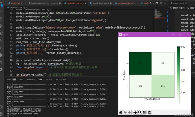
yp = model.predict(x).reshape(len(y))
yp = np.around(yp,0).astype(int) #转换为整型
from cm_plot import *  # 导入自行编写的混淆矩阵可视化函数

cm_plot(y,yp).show()  # 显示混淆矩阵可视化结果

cm_plot函数：

#-*- coding: utf-8 -*-
def cm_plot(y, yp):
  
  from sklearn.metrics import confusion_matrix #导入混淆矩阵函数

  cm = confusion_matrix(y, yp) #混淆矩阵
  
  import matplotlib.pyplot as plt #导入作图库
  plt.matshow(cm, cmap=plt.cm.Greens) #画混淆矩阵图，配色风格使用cm.Greens，更多风格请参考官网。
  plt.colorbar() #颜色标签
  
  for x in range(len(cm)): #数据标签
    for y in range(len(cm)):
      plt.annotate(cm[x,y], xy=(x, y), horizontalalignment='center', verticalalignment='center')
  
  plt.ylabel('True label') #坐标轴标签
  plt.xlabel('Predicted label') #坐标轴标签
  return plt

二、用机器学习相关算法搭建

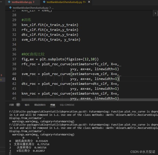
1、支持向量机（SVM）、随机森林、决策树、KNN（K邻近）

ROC曲线：

得分：

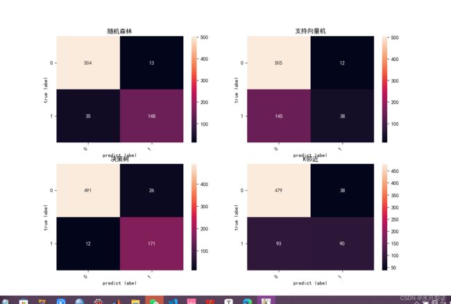
混淆矩阵：

决策树：

完整代码：

import pandas as pd
import time
import numpy as np
import seaborn as sns
import matplotlib.pyplot as plt 
from sklearn.model_selection import train_test_split
from sklearn.tree import DecisionTreeClassifier as DTC
from sklearn.ensemble import RandomForestClassifier as RFC
from sklearn import svm
from sklearn import tree
from sklearn.metrics import confusion_matrix
from sklearn.metrics import accuracy_score
from sklearn.metrics import roc_curve, auc
from sklearn.neighbors import KNeighborsClassifier as KNN
#导入plot_roc_curve,roc_curve和roc_auc_score模块
from sklearn.metrics import plot_roc_curve,roc_curve,auc,roc_auc_score
filePath = 'C:/Users/86188/Desktop/Python数据挖掘与数据分析/My work/data2/bankloan2.xls'
data = pd.read_excel(filePath)
x = data.iloc[:,:8]
y = data.iloc[:,8]
x_train, x_test, y_train, y_test = train_test_split(x, y, test_size=0.2, random_state=100)

#模型
svm_clf = svm.SVC()#支持向量机
dtc_clf = DTC(criterion='entropy')#决策树
rfc_clf = RFC(n_estimators=10)#随机森林
knn_clf = KNN()#K邻近

#训练
knn_clf.fit(x_train,y_train)
rfc_clf.fit(x_train,y_train)
dtc_clf.fit(x_train,y_train)
svm_clf.fit(x_train, y_train)


#ROC曲线比较
fig,ax = plt.subplots(figsize=(12,10))
rfc_roc = plot_roc_curve(estimator=rfc_clf, X=x, 
                        y=y, ax=ax, linewidth=1)
svm_roc = plot_roc_curve(estimator=svm_clf, X=x, 
                        y=y, ax=ax, linewidth=1)
dtc_roc = plot_roc_curve(estimator=dtc_clf, X=x,
                        y=y, ax=ax, linewidth=1)
knn_roc = plot_roc_curve(estimator=knn_clf, X=x,
                        y=y, ax=ax, linewidth=1)
ax.legend(fontsize=12)
plt.show()

#模型评价
rfc_yp = rfc_clf.predict(x)
rfc_score = accuracy_score(y, rfc_yp)
svm_yp = svm_clf.predict(x)
svm_score = accuracy_score(y, svm_yp)
dtc_yp = dtc_clf.predict(x)
dtc_score = accuracy_score(y, dtc_yp)
knn_yp = knn_clf.predict(x)
knn_score = accuracy_score(y, knn_yp)
score = {"随机森林得分":rfc_score,"支持向量机得分":svm_score,"决策树得分":dtc_score,"K邻近得分":knn_score}
score = sorted(score.items(),key = lambda score:score[0],reverse=True)
print(pd.DataFrame(score))

#中文标签、负号正常显示
plt.rcParams['font.sans-serif'] = ['SimHei']
plt.rcParams['axes.unicode_minus'] = False

#绘制混淆矩阵
figure = plt.subplots(figsize=(12,10))
plt.subplot(2,2,1)
plt.title('随机森林')
rfc_cm = confusion_matrix(y, rfc_yp)
heatmap = sns.heatmap(rfc_cm, annot=True, fmt='d')
heatmap.yaxis.set_ticklabels(heatmap.yaxis.get_ticklabels(), rotation=0, ha='right')
heatmap.xaxis.set_ticklabels(heatmap.xaxis.get_ticklabels(), rotation=45, ha='right')
plt.ylabel("true label")
plt.xlabel("predict label")

plt.subplot(2,2,2)
plt.title('支持向量机')
svm_cm = confusion_matrix(y, svm_yp)
heatmap = sns.heatmap(svm_cm, annot=True, fmt='d')
heatmap.yaxis.set_ticklabels(heatmap.yaxis.get_ticklabels(), rotation=0, ha='right')
heatmap.xaxis.set_ticklabels(heatmap.xaxis.get_ticklabels(), rotation=45, ha='right')
plt.ylabel("true label")
plt.xlabel("predict label")

plt.subplot(2,2,3)
plt.title('决策树')
dtc_cm = confusion_matrix(y, dtc_yp)
heatmap = sns.heatmap(dtc_cm, annot=True, fmt='d')
heatmap.yaxis.set_ticklabels(heatmap.yaxis.get_ticklabels(), rotation=0, ha='right')
heatmap.xaxis.set_ticklabels(heatmap.xaxis.get_ticklabels(), rotation=45, ha='right')
plt.ylabel("true label")
plt.xlabel("predict label")

plt.subplot(2,2,4)
plt.title('K邻近')
knn_cm = confusion_matrix(y, knn_yp)
heatmap = sns.heatmap(knn_cm, annot=True, fmt='d')
heatmap.yaxis.set_ticklabels(heatmap.yaxis.get_ticklabels(), rotation=0, ha='right')
heatmap.xaxis.set_ticklabels(heatmap.xaxis.get_ticklabels(), rotation=45, ha='right')
plt.ylabel("true label")
plt.xlabel("predict label")
plt.show()

#画出决策树
import pandas as pd
import os
os.environ["PATH"] += os.pathsep + 'D:/软件下载安装/Graphviz/bin'
from sklearn.tree import export_graphviz
x = pd.DataFrame(x)

with open(r"C:/Users/86188/Desktop/Python数据挖掘与数据分析/My work/tmp/banklodan_tree.dot", 'w') as f:
    export_graphviz(dtc_clf, feature_names = x.columns, out_file = f)
    f.close()
    
from IPython.display import Image  
from sklearn import tree
import pydotplus 
dot_data = tree.export_graphviz(dtc_clf, out_file=None,  #regr_1 是对应分类器
                         feature_names=x.columns,   #对应特征的名字
                         class_names= ['不违约','违约'],    #对应类别的名字
                         filled=True, rounded=True,  
                         special_characters=True)  

#让graphviz显示中文用"MicrosoftYaHei"代替'helvetica'
graph = pydotplus.graph_from_dot_data(dot_data.replace('helvetica',"MicrosoftYaHei"))  
graph.write_png('C:/Users/86188/Desktop/Python数据挖掘与数据分析/My work/tmp/banklodan_tree.png')    #保存图像
Image(graph.create_png()) 

结论：

显然，决策树和随机森林的效果最好，总体上都比神经网络的要好

三、资料链接

我的代码和数据
提取码：0325

四、参考链接：

二分类评分
Sequential序贯模型
ROC曲线绘制
Grapviz显示中文