【cs231n Lesson3】Optimization, Gradient descent

个人学习笔记
date：2023.01.03
参考网站：cs231n官方笔记

Optimization

损失函数让我们知道权重矩阵$\mathbf{W}$的质量；
优化的目的则是让我们找到合适的$\mathbf{W}$使得损失函数更小。

$（一）随机查找（bad）$

bestloss = float("inf") # Python assigns the highest possible float value
for num in range(1000):
  W = np.random.randn(10, 3073) * 0.0001 # generate random parameters
  loss = L(X_train, Y_train, W) # get the loss over the entire training set
  if loss < bestloss: # keep track of the best solution
    bestloss = loss
    bestW = W
  print 'in attempt %d the loss was %f, best %f' % (num, loss, bestloss)

并将使损失函数最小的权重矩阵用到测试集

# Assume X_test is [3073 x 10000], Y_test [10000 x 1]
scores = Wbest.dot(Xte_cols) # 10 x 10000, the class scores for all test examples
# find the index with max score in each column (the predicted class)
Yte_predict = np.argmax(scores, axis = 0)
# and calculate accuracy (fraction of predictions that are correct)
np.mean(Yte_predict == Yte)
# returns 0.1555

但事实上，找到最佳的$\mathbf{W}$很难，但是从一个随机矩阵开始，每一次都将其优化就不那么难。

Our strategy will be to start with random weights and iteratively refine them over time to get lower loss

$（二）随机局部查找（bad）$

从随机矩阵$\mathbf{W}$开始，加上随机产生的干扰项$\delta W$ ,如果损失函数更小，则更新之。

W = np.random.randn(10, 3073) * 0.001 # generate random starting W
bestloss = float("inf")
for i in range(1000):
  step_size = 0.0001
  Wtry = W + np.random.randn(10, 3073) * step_size
  loss = L(Xtr_cols, Ytr, Wtry)
  if loss < bestloss:
    W = Wtry
    bestloss = loss
  print 'iter %d loss is %f' % (i, bestloss)

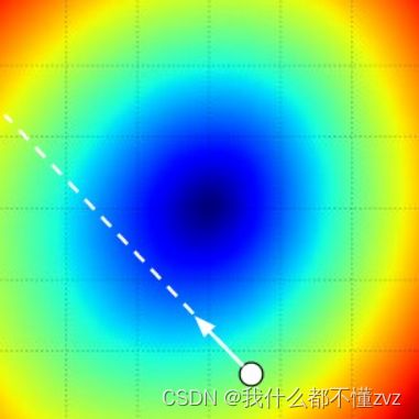
$（三）梯度下降gradientdescent$

数学上，计算出损失函数的梯度，即可知道增长速度最快的方向，取反既是减小速度最快的方向。

在1-d 空间，某一点的梯度既是该点的导数，表达式为
$$\frac{dy}{dx}=li{m}_{h\to 0}\frac{f(x+h)-f(x)}{h}$$

$通过有限差分逼近方法计算梯度$
让每个维度的都移动很小的距离，然后计算导数（梯度）

def eval_numerical_gradient(f, x):
  """
  a naive implementation of numerical gradient of f at x
  - f should be a function that takes a single argument
  - x is the point (numpy array) to evaluate the gradient at
  """

  fx = f(x) # evaluate function value at original point
  grad = np.zeros(x.shape)
  h = 0.00001

  # iterate over all indexes in x
  it = np.nditer(x, flags=['multi_index'], op_flags=['readwrite'])
  while not it.finished:

    # evaluate function at x+h
    ix = it.multi_index
    old_value = x[ix]
    x[ix] = old_value + h # increment by h
    fxh = f(x) # evalute f(x + h)
    x[ix] = old_value # restore to previous value (very important!)

    # compute the partial derivative
    grad[ix] = (fxh - fx) / h # the slope
    it.iternext() # step to next dimension

  return grad

• np.nditer(x,flags=['multi_index'],op_flags=['readwrite'] 生成迭代器对象，遍历数组。flags为multi_index表示跟踪多个迭代维度
• it.finished表示末端
• it.multi_index表示多维迭代
  参考：https://blog.csdn.net/weixin_43868107/article/details/102647760

通常使用中心差分公式来计算梯度会更好：
$$[f(x+h)-f(x-h)]/2h$$

通过梯度来更新权重矩阵：

def CIFAR10_loss_fun(W):
  return L(X_train, Y_train, W)

W = np.random.rand(10, 3073) * 0.001 # random weight vector
df = eval_numerical_gradient(CIFAR10_loss_fun, W) # get the gradient

loss_original = CIFAR10_loss_fun(W) # the original loss
print 'original loss: %f' % (loss_original, )

# lets see the effect of multiple step sizes
for step_size_log in [-10, -9, -8, -7, -6, -5,-4,-3,-2,-1]:
  step_size = 10 ** step_size_log
  W_new = W - step_size * df # new position in the weight space
  loss_new = CIFAR10_loss_fun(W_new)
  print 'for step size %f new loss: %f' % (step_size, loss_new)

# prints:
# original loss: 2.200718
# for step size 1.000000e-10 new loss: 2.200652
# for step size 1.000000e-09 new loss: 2.200057
# for step size 1.000000e-08 new loss: 2.194116
# for step size 1.000000e-07 new loss: 2.135493
# for step size 1.000000e-06 new loss: 1.647802
# for step size 1.000000e-05 new loss: 2.844355
# for step size 1.000000e-04 new loss: 25.558142
# for step size 1.000000e-03 new loss: 254.086573
# for step size 1.000000e-02 new loss: 2539.370888
# for step size 1.000000e-01 new loss: 25392.214036

• 我们需要朝着梯度的负方向前进，因为我们希望损失函数下降而不是上升
• 选取一个正确的step size或者说learning rate是很关键的。学习率太小，我们可以取得很小的进步，也可能陷入到局部极值的困境中；学习率太大，就像上面数据一样，可能造成更大的损失值。
  
• 效率问题：一般神经网络有非常多的参数，我们需要计算每一个参数的梯度然后做一个小小的更新是非常低性价比的。

$通过微积分方法计算梯度$

• 有限差分方法计算梯度是不完全准确的（h取值为很小的值，但是公式中h趋于0），并且耗时高。
• 微积分方法可以准确表达梯度，但是应用中容易出错，所以需要用有限差分方法来进行梯度检查。

比如SVM损失函数
$$L_i=\sum _{j\ne y_i}[max(0,w_j^T{x}_i-w_{y_i}^T{x}_i+\Delta )]$$

正确结果一行的梯度为
$$gra{d}_{w_{y_i}}=-(\sum _{j\ne y_i}1(w_j^T{x}_i-w_{y_i}^T{x}_i+\Delta >0))x_i$$

其他行的梯度为：
$$gra{d}_{w_{y_i}}=1(w_j^T{x}_i-w_{y_i}^T{x}_i+\Delta >0)x_i$$

$梯度下降更新参数$
模板如下

while True:
  weights_grad = evaluate_gradient(loss_fun, data, weights)
  weights += - step_size * weights_grad # perform parameter update

Mini-batch gradient descent:
通过会取很小的batch来进行梯度估算，然后更新参数。通过取32/64/128/256个元素（2的幂次，because many vectorized operation implementations work faster when their inputs are sized in powers of 2.）

while True:
  data_batch = sample_training_data(data, 256) # sample 256 examples
  weights_grad = evaluate_gradient(loss_fun, data_batch, weights)
  weights += - step_size * weights_grad # perform parameter update

为什么可以使用mini-batch计算梯度来替代整个训练集计算得来的梯度：

1. 实际上训练集每一个类都有一张unique的图像，然后同一类下的其他图像都是这一个图像的identical copies。所以我们计算同一类下所有图像的梯度是相同的。并且我们计算训练集所有图像损失的均值，会和mini-batch的损失均值一样。所以可以很好估算整个训练集的梯度。
2. 如果mini-batch只包含一个例子，这一过程叫Stochastic Gradient Descent（SGD）随机梯度下降，其实不常见，比较低效（计算100个例子的梯度和计算1个例子的梯度100次，由于矢量化，前者更好）