python实现决策树分类 mnist数据集

1.原理介绍

原理：决策树分类器是一种有监督的机器学习方法。决策树方法不能用于缺少值的数据集，因为我们知道这个数据集没有这个问题，我们不需要对它进行任何计算。决策树的基本工作原理是，使用递归二进制拆分创建一棵大树，然后选择一小群子树，使用成本复杂度修剪，并在每个子树中执行交叉验证，以选择一个错误较少的子树

2.实验过程

2.1导入库

# 标准库
import numpy as np
import pandas as pd

# 可视化的库
import matplotlib.pyplot as plt
import seaborn as sns

# 建模和机器学习
from sklearn.tree import DecisionTreeClassifier
from sklearn.metrics import confusion_matrix,accuracy_score, classification_report
from sklearn.model_selection import train_test_split

2.2加载数据集

df = pd.read_csv('D:\\train.csv')# 导入训练集
df.head()  # 查看数据集前五行

运行结果：

	label	pixel0	pixel1	pixel2	pixel3	pixel4	pixel5	pixel6	pixel7	pixel8	...	pixel774	pixel775	pixel776	pixel777	pixel778	pixel779	pixel780	pixel781	pixel782	pixel783
0	1	0	0	0	0	0	0	0	0	0	...	0	0	0	0	0	0	0	0	0	0
1	0	0	0	0	0	0	0	0	0	0	...	0	0	0	0	0	0	0	0	0	0
2	1	0	0	0	0	0	0	0	0	0	...	0	0	0	0	0	0	0	0	0	0
3	4	0	0	0	0	0	0	0	0	0	...	0	0	0	0	0	0	0	0	0	0
4	0	0	0	0	0	0	0	0	0	0	...	0	0	0	0	0	0	0	0	0	0

5 rows × 785 columns

df.shape

运行结果：

(42000, 785)

2.3可视化目标分布情况

# 对标签进行排序并且做出柱状图
df['label'].value_counts().sort_index().plot(kind='bar', figsize=(10, 6), rot=0)
plt.title('Class distribution for the MNIST Dataset', fontsize=20) 
plt.xticks(fontsize=14)  
plt.yticks(fontsize=14)  
plt.xlabel('Class', fontsize=16)  
plt.ylabel('Frequency', fontsize=16)  

运行结果：

Text(0, 0.5, ‘Frequency’)

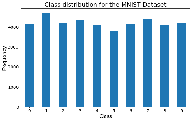
上面的可视化显示目标分布非常均匀，所以不需要执行额外的预处理。

2.4对训练变量和目标变量的数据进行分解

X=df.iloc[:,1:]  # 选择所有行和列，但排除列1
print("features shape: ", X.shape)
y=df['label']  # 将label列作为预测值
print("Target shape: ", y.shape)

运行结果：
features shape: (42000, 784)
Target shape: (42000,)

2.5划分训练集和验证集

# 划分数据集
X_train, X_valid, y_train, y_valid = train_test_split(X, y,test_size = 0.3,random_state=0)

# 将训练集与验证集的尺度进行输出
print('Shape of X_train:', X_train.shape)
print('Shape of y_train:', y_train.shape)
print('Shape of X_valid:', X_valid.shape)
print('Shape of y_valid:', y_valid.shape)

运行结果：
Shape of X_train: (29400, 784)
Shape of y_train: (29400,)
Shape of X_valid: (12600, 784)
Shape of y_valid: (12600,)

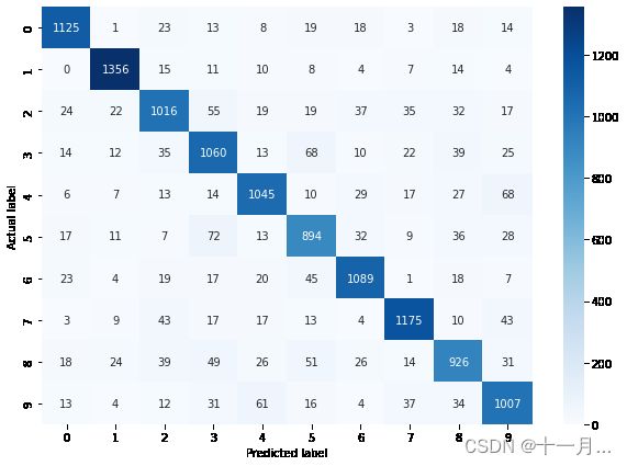
2.6训练模型和结果

dtModel = DecisionTreeClassifier()  # 建立模型
dtModel.fit(X_train,y_train)  
prediction = dtModel.predict(X_valid)  
plt.figure(figsize=(10,7)) 
cm = confusion_matrix(y_valid,  prediction) 

ax = sns.heatmap(cm, annot=True, fmt="d",cmap='Blues')  
plt.ylabel('Actual label')  # x轴标题
plt.xlabel('Predicted label')  # y轴标题

acc = accuracy_score(y_valid,prediction)  
print(f"Sum Axis-1 as Classification accuracy: {acc* 100}")

运行结果：

Sum Axis-1 as Classification accuracy: 84.86507936507937

# print ("Accuracy on Training Data：{0:.2f}%".format(dtModel.score(X_train, y_train)*100))
print ("Accuracy on Test Data：{0:.2f}%".format(dtModel.score(X_valid, y_valid)*100))

运行结果：

Accuracy on Test Data：84.52%

# 对于分类算法还可以观察accuracy，Precision，Recall，F-score等
print("\nClassification Report:")
print(classification_report(y_valid, prediction))

运行结果：

Classification Report:
              precision    recall  f1-score   support

           0       0.91      0.91      0.91      1242
           1       0.93      0.94      0.94      1429
           2       0.82      0.79      0.80      1276
           3       0.79      0.81      0.80      1298
           4       0.85      0.85      0.85      1236
           5       0.76      0.80      0.78      1119
           6       0.87      0.87      0.87      1243
           7       0.88      0.87      0.87      1334
           8       0.81      0.77      0.79      1204
           9       0.81      0.82      0.82      1219

    accuracy                           0.85     12600
   macro avg       0.84      0.84      0.84     12600
weighted avg       0.85      0.85      0.85     12600

2.7进行测试

df1 = pd.read_csv('D:\\test.csv')  # 导入测试集
df1.head()  

运行结果：

	pixel0	pixel1	pixel2	pixel3	pixel4	pixel5	pixel6	pixel7	pixel8	pixel9	...	pixel774	pixel775	pixel776	pixel777	pixel778	pixel779	pixel780	pixel781	pixel782	pixel783
0	0	0	0	0	0	0	0	0	0	0	...	0	0	0	0	0	0	0	0	0	0
1	0	0	0	0	0	0	0	0	0	0	...	0	0	0	0	0	0	0	0	0	0
2	0	0	0	0	0	0	0	0	0	0	...	0	0	0	0	0	0	0	0	0	0
3	0	0	0	0	0	0	0	0	0	0	...	0	0	0	0	0	0	0	0	0	0
4	0	0	0	0	0	0	0	0	0	0	...	0	0	0	0	0	0	0	0	0	0

5 rows × 784 columns

df1.shape

运行结果：

(28000, 784)

def print_testimage(index):   
    some_digit = df1.iloc[index].values  # 按照索引取出图片
    some_digit_img = some_digit.reshape(28,28)  
    plt.imshow(some_digit_img,'binary')  # 展示

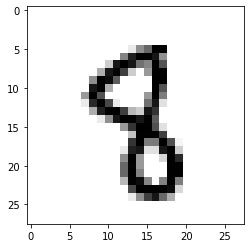
2.8一个随机预测

print_testimage(2000) # 查看第2000张图片

运行结果：

2.9抽查预测是否正确。将预测标绘为标签

figr,axes=plt.subplots(figsize=(10,10),ncols=3,nrows=3) 
axes=axes.flatten()  
for i in range(0,9):  # 循环
    jj=np.random.randint(0,X_valid.shape[0])          #挑选一个随机图片
    axes[i].imshow(X_valid.iloc[[jj]].values.reshape(28,28))  
    axes[i].set_title('predicted: '+str(dtModel.predict(X_valid.iloc[[jj]])[0]))

运行结果：

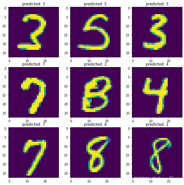
上面介绍了随机预测一张图片和预测多张图片的方法，大家可以任意选择

2.10使用网格搜索法进行调参

## 从sklearn库中导入网格调参函数
from sklearn.model_selection import GridSearchCV

## 定义参数取值范围

parameters = {'splitter':('best','random')
              ,'criterion':("gini","entropy")
              ,"max_depth":[*range(1,10)]
              ,'min_samples_leaf':[*range(1,50,1)]
}
model = DecisionTreeClassifier()

## 进行网格搜索
clf = GridSearchCV(model, parameters, cv=3, scoring='accuracy',verbose=3, n_jobs=-1)
clf = clf.fit(X_train, y_train)

运行结果：
Fitting 3 folds for each of 1764 candidates, totalling 5292 fits

clf.best_params_  # 得到最好的参数

运行结果：
{‘criterion’: ‘entropy’,
‘max_depth’: 9,
‘min_samples_leaf’: 1,
‘splitter’: ‘best’}

# 使用最好的参数再一次输出
model = DecisionTreeClassifier(criterion='entropy',max_depth=9,min_samples_leaf=1,splitter='best')
model.fit(X_train,y_train) 
prediction = model.predict(X_valid)   
acc = accuracy_score(y_valid,prediction)  
print(f"Sum Axis-1 as Classification accuracy: {acc* 100}")

运行结果：
Sum Axis-1 as Classification accuracy: 84.92857142857143

参考

1. 决策树的原理