V2V网络灵敏度分析(Matlab代码实现）

           目录

1 概述

2 运行结果

3 参考文献

‍4 Matlab代码

---

1 概述

灵敏度分析是研究与分析一个系统（或模型）的状态或输出变化对系统参数或周围条件变化的敏感程度的方法。在最优化方法中经常利用灵敏度分析来研究原始数据不准确或发生变化时最优解的稳定性。通过灵敏度分析还可以决定哪些参数对系统或模型有较大的影响。因此，灵敏度分析几乎在所有的运筹学方法以及在对各种方案进行评价时都是很重要的。特别要注意的是，在热传递问题中，一般要考虑热辐射、热传导以及热对流对温度场的影响。

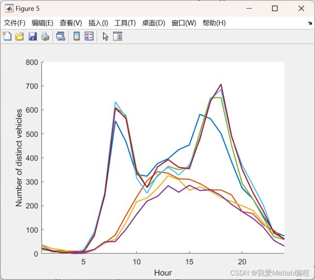
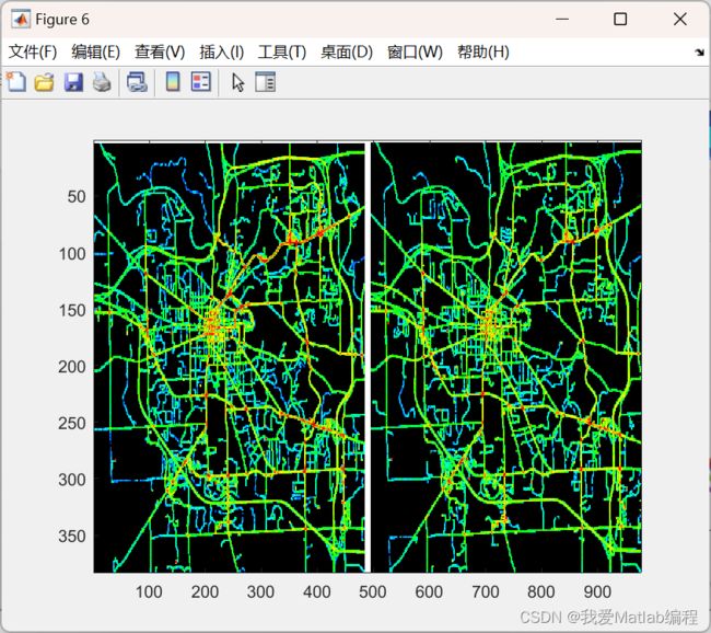
2 运行结果

 

 

 

 

3 参考文献

[1] Macheng Shen, Ding Zhao, and Jing Sun. "The Impact of Road Configuration in V2V-based Cooperative Localization: Mathematical Analysis and Real-world Evaluation." arXiv preprint arXiv:1705.00568 (2017).

For detail, see the comments in 'main.m'. To calculate the CMM error over Ann Arbor (corresponding to fannarbor=1), four data files are required, ask [email protected] for the data files.

‍4 Matlab代码

主函数部分代码：

%% Add path of data and figure

data_path = './data_and_figure';
addpath(data_path)

%% Main
% Control parameter:
fsim=0; % fsim=1: run simulation to generate data; fsim=1: load data from file
fplot=1; %fplot=1: plot data
fsave=0; %fsave=1: save data to .mat file
fannarbor=0; %fannarbor=1: predict CMM error in ann arbor, require traffice flow data file

if fsim==1
    n=3:12;
    E_X=pi^2*0.09/12./log(n);
    [n_MC,E_MC]=MC_analytic(0.3);
    
    n4=10:50;
    E_X4=8/9./n4+1.5*0.09./n4;
    [n_MC4,E_MC4]=mean_err_MC_uniform(0.09);
    
    [n_ort,E_ort]=MC_analytic(1);
    [n_uni,E_uni]=mean_err_MC_uniform(1);
end

if fsim==0
    load predicted_error.mat;
end

if fplot==1
    
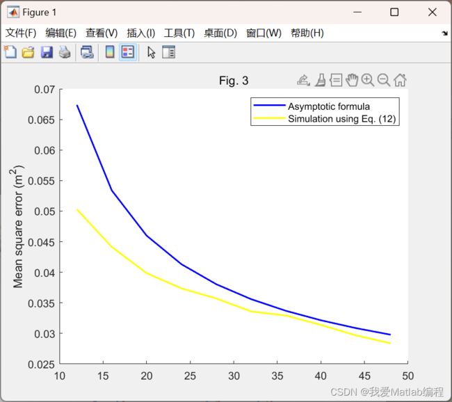
    figure
    hold on;
    plot(n*4,E_X,'b','LineWidth',1.5)
    plot(n_MC,E_MC,'y','LineWidth',1.5)
    legend('Asymptotic formula','Simulation using Eq. (12)')
    ylabel('Mean square error (m^2)')
    title('Fig. 3')
    
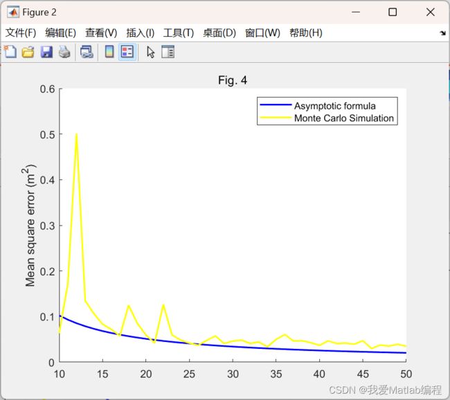
    figure
    hold on;
    plot(n4,E_X4,'b','LineWidth',1.5)
    plot(n_MC4,E_MC4,'y','LineWidth',1.5)
    legend('Asymptotic formula','Monte Carlo Simulation')
    ylabel('Mean square error (m^2)')
    title('Fig. 4')
    
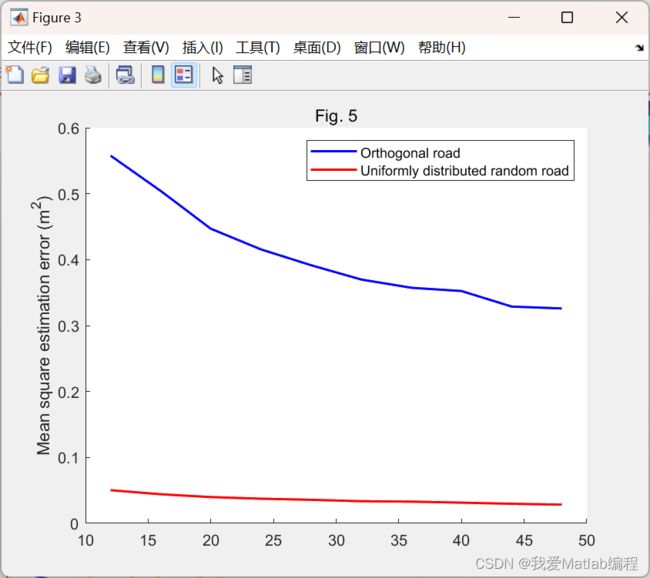
    figure
    hold on;
    loglog(n_ort,E_ort,'b','LineWidth',1.5)
    loglog(n_MC,E_MC,'r','LineWidth',1.5)
    legend('Orthogonal road','Uniformly distributed random road')
    ylabel('Mean square estimation error (m^2)')
    title('Fig. 5')
    
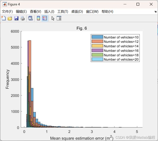
    figure
    hold on;
    for k=10:2:20
        m=0;
        for i=1:10000
            angle=rand(1,k)*2*pi;
            temp=square_error(angle,2,0.5,0);
            if temp<5
                er(m+1)=temp;
                m=m+1;
            end
        end
        histogram(er);
    end