神经网络求解偏微分方程代码分析

在我分享了我的神经网络求解微分方程的代码后，很多志同道合的朋友与我进行了交流。下面把我求解偏微分方程的代码分享出来，主要是分享代码思路。这个代码是在求解常微分方程的基础上进行的修改，现在看来有些语句可以换成更高级的表达。若有更好的表达方式欢迎评论/私信！

运行环境：python3.6 + tensorflow1.2.1 + CPU
若要tensorflow2.0及以上的版本运行需要添加一行代码

数学问题

程序想要解决的数学问题是

其中求解区域是

对于偏微分方程的 Dirichlet 边界条件由以下方程给出：

这个微分方程有显式解析解，解析解为：

求解后可以与标准的解析解对比结果。

代码展示

import os
os.environ['TF_CPP_MIN_LOG_LEVEL'] = '2'
#导入相关支持文件包
import tensorflow as tf
import matplotlib.pyplot as plt
import numpy as np
import math
from mpl_toolkits.mplot3d import Axes3D
#产生数据，数据
x_train_1 = np.linspace(0, 1, 10)#生成[0,1]区间10个点
x_train_2 = np.linspace(0, 1, 10)#生成[0,1]区间10个点
input_num = []
for i in range(len(x_train_1)):
    for j in range(len(x_train_2)):
        input_num.append([x_train_1[i], x_train_2[j]])
input_num = np.array(input_num)
input_x1, input_x2 = np.expand_dims(input_num[:, 0], 1), np.expand_dims(input_num[:, 1], 1)

y_trail = np.exp(-1*input_x1)*(input_x1+input_x2**3)
X2, X1 = np.meshgrid(x_train_1, x_train_2)#使用X1,X2画3维图用

fig = plt.figure("解析解图像")
ax = fig.gca(projection='3d')
ax.plot_surface(X1, X2, y_trail.reshape(10, 10), rstride=1, cstride=1, cmap=plt.get_cmap('rainbow'))

def fwd_gradients(Y, x):
    dummy = tf.ones_like(Y)
    G = tf.gradients(Y, x, grad_ys=dummy, colocate_gradients_with_ops=True)[0]
    Y_x = tf.gradients(G, dummy, colocate_gradients_with_ops=True)[0]
    return Y_x
def act(x):
    return x*tf.nn.sigmoid(x)
A = tf.placeholder("float", [None, 1])#一次传入100个点[100,1]
B = tf.placeholder("float", [None, 1])#一次传入100个点[100,1]
W1_1 = tf.Variable(tf.random_normal([1, 10])*0.01)
W1_2 = tf.Variable(tf.random_normal([1, 10])*0.01)
b = tf.Variable(tf.zeros([10])+0.01)
y1 = act(tf.matmul(A, W1_1)+tf.matmul(B, W1_2)+b)#sigmoid激活函数y1的形状[100,10]
W2 = tf.Variable(tf.random_normal([10, 1])*0.01)
y = tf.matmul(y1, W2)#网络的输出[100,1]
lq = tf.exp(-1*A)*(A-2+B**3+6*B)
dif_A = fwd_gradients(y, A)
dif_B = fwd_gradients(y, B)
dif_AA = fwd_gradients(dif_A, A)
dif_BB = fwd_gradients(dif_B, B)
sum = 0
for i in range(10):
    sum += (y[i, 0]-x_train_2[i]**3)**2
for i in range(10):
    sum += (y[i+10, 0]-(1+(x_train_2[i])**3)*math.exp(-1))**2
for i in range(10):
    sum += (y[i*10, 0]-x_train_2[i]*math.exp(-1*x_train_2[i]))**2
for i in range(10):
    sum += (y[i*10+9, 0]-(x_train_2[i]+1)*math.exp(-1*x_train_2[i]))**2
t_loss = (dif_AA+dif_BB-lq)**2#常微分方程F的平方
loss = tf.reduce_mean(t_loss)+sum#未加边界条件！！！！！！！
train_step = tf.train.AdamOptimizer(0.001).minimize(loss)#Adam优化器训练网络参数
init = tf.global_variables_initializer()
with tf.Session() as sess:
    sess.run(init)
    for i in range(50000):#训练50000次
        sess.run(train_step, feed_dict={A: input_x1, B: input_x2})
        if i % 50 == 0:
            total_loss = sess.run(loss, feed_dict={A: input_x1, B: input_x2})
            print("loss={}".format(total_loss))
    output = sess.run(y, feed_dict={A: input_x1, B: input_x2})
    output1 = sess.run(t_loss, feed_dict={A: input_x1, B: input_x2})
    fig = plt.figure("预测曲面")
    bx = fig.gca(projection='3d')
    bx.plot_surface(X1, X2, output.reshape(10, 10), rstride=1, cstride=1, cmap=plt.get_cmap('rainbow'))
    fig = plt.figure("y-y_")
    cset = plt.contourf(X1, X2, (output-y_trail).reshape(10, 10),cmap=plt.get_cmap('rainbow'))
    plt.contour(X1, X2, (output-y_trail).reshape(10, 10))
    plt.colorbar(cset)
    plt.show()

代码分析

程序首先导入相关的支持包文件，然后在[0,1]的区间上产生等距的10个采样点。两个维度分别产生了10个采样点后就能在xoy面上产生100个组合采样点。

定义的act()方法是激活函数swish。这个函数在求解二阶偏微分方程方面有着较好的性质。除了swish函数，tanh函数也可做为该网络的激活函数。求解偏微分方程涉及到输出对输入的微分，ReLu函数的二阶微分后全都为0，故不能用作激活函数。

fwd_gradients(Y, x)功能是求出Y对输入x的微分，返回值即为微分后的值。

结果展示

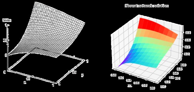
左图为函数的解析解绘制的图像，右图为神经网络绘制的图像。可以看出通过上述的神经网络能够较好的拟合解析解的结果。