多标签分类 评价指标
Metrics play quite an important role in the field of Machine Learning or Deep Learning. We start the problems with metric selection as to know the baseline score of a particular model. In this blog, we look into the best and most common metrics for Multi-Label Classification and how they differ from the usual metrics.
指标在机器学习或深度学习领域中扮演着非常重要的角色。 我们从度量选择开始着手,以了解特定模型的基线得分。 在此博客中,我们研究了“多标签分类”的最佳和最常用指标,以及它们与通常的指标有何不同。
Let me get into what is Multi-Label Classification just in case you need it. If we have data about the features of a dog and we had to predict which breed and pet category it belonged to.
让我进入什么是多标签分类,以防万一您需要它。 如果我们有关于狗的特征的数据,并且我们必须预测它属于哪个品种和宠物。
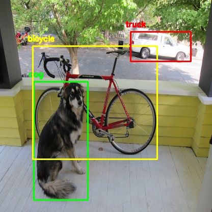
In the case of Object Detection, Multi-Label Classification gives us the list of all the objects in the image as follows. We can see that the classifier detects 3 objects in the image. It can be made into a list as follows [1 0 1 1] if the total number of trained objects are 4 ie. [dog, human, bicycle, truck].
在对象检测的情况下,多标签分类为我们提供了图像中所有对象的列表,如下所示。 我们可以看到分类器检测到图像中的3个对象。 如果训练对象的总数为4,即[1 0 1 1],则可以将其列为以下列表。 [狗,人,自行车,卡车]。
This kind of classification is known as Multi-Label Classification.
这种分类称为多标签分类。
The most common metrics that are used for Multi-Label Classification are as follows:
用于多标签分类的最常见指标如下:
- Precision at k k精度
- Avg precision at k平均精度(k)
- Mean avg precision at k k的平均平均精度
- Sampled F1 Score采样的F1分数
Let’s get into the details of these metrics.
让我们详细了解这些指标。
k精度(P @ k): (Precision at k (P@k):)
Given a list of actual classes and predicted classes, precision at k would be defined as the number of correct predictions considering only the top k elements of each class divided by k. The values range between 0 and 1.
给定实际类别和预测类别的列表,将在k处的精度定义为仅考虑每个类别的前k个元素除以k得出的正确预测数。 取值范围是0到1。
Here is an example as explaining the same in code:
这是一个解释相同代码的示例:
def patk(actual, pred, k):
	#we return 0 if k is 0 because
	#   we can't divide the no of common values by 0
	if k == 0:
		return 0


	#taking only the top k predictions in a class
	k_pred = pred[:k]


	#taking the set of the actual values
	actual_set = set(actual)


	#taking the set of the predicted values
	pred_set = set(k_pred)


	#taking the intersection of the actual set and the pred set
		# to find the common values
	common_values = actual_set.intersection(pred_set)


	return len(common_values)/len(pred[:k])


#defining the values of the actual and the predicted class
y_true = [1 ,2, 0]
y_pred = [1, 1, 0]


if __name__ == "__main__":
    print(patk(y_true, y_pred,3))
Running the following code, we get the following result.
运行以下代码,我们得到以下结果。
0.6666666666666666In this case, we got the value of 2 as 1, thus resulting in the score going down.
在这种情况下,我们将2的值设为1,从而导致得分下降。
K处的平均精度(AP @ k): (Average Precision at K (AP@k):)
It is defined as the average of all the precision at k for k =1 to k. To make it more clear let’s look at some code. The values range between 0 and 1.
它定义为k = 1至k时k处所有精度的平均值。 为了更加清楚,让我们看一些代码。 取值范围是0到1。
import numpy as np
import pk


def apatk(acutal, pred, k):
	#creating a list for storing the values of precision for each k
	precision_ = []
	for i in range(1, k+1):
		#calculating the precision at different values of k
		#      and appending them to the list
		precision_.append(pk.patk(acutal, pred, i))


	#return 0 if there are no values in the list
	if len(precision_) == 0:
		return 0


	#returning the average of all the precision values
	return np.mean(precision_)


#defining the values of the actual and the predicted class
y_true = [[1,2,0,1], [0,4], [3], [1,2]]
y_pred = [[1,1,0,1], [1,4], [2], [1,3]]


if __name__ == "__main__":
	for i in range(len(y_true)):
		for j in range(1, 4):
			print(
				f"""
				y_true = {y_true[i]}
				y_pred = {y_pred[i]}
				AP@{j} = {apatk(y_true[i], y_pred[i], k=j)}
				"""
			)
Here we check for the AP@k from 1 to 4. We get the following output.
在这里,我们检查从1到4的AP @ k。我们得到以下输出。
y_true = [1, 2, 0, 1]
				y_pred = [1, 1, 0, 1]
				AP@1 = 1.0


				y_true = [1, 2, 0, 1]
				y_pred = [1, 1, 0, 1]
				AP@2 = 0.75


				y_true = [1, 2, 0, 1]
				y_pred = [1, 1, 0, 1]
				AP@3 = 0.7222222222222222


				y_true = [0, 4]
				y_pred = [1, 4]
				AP@1 = 0.0


				y_true = [0, 4]
				y_pred = [1, 4]
				AP@2 = 0.25


				y_true = [0, 4]
				y_pred = [1, 4]
				AP@3 = 0.3333333333333333


				y_true = [3]
				y_pred = [2]
				AP@1 = 0.0


				y_true = [3]
				y_pred = [2]
				AP@2 = 0.0


				y_true = [3]
				y_pred = [2]
				AP@3 = 0.0


				y_true = [1, 2]
				y_pred = [1, 3]
				AP@1 = 1.0


				y_true = [1, 2]
				y_pred = [1, 3]
				AP@2 = 0.75


				y_true = [1, 2]
				y_pred = [1, 3]
				AP@3 = 0.6666666666666666
This gives us a clear understanding of how the code works.
这使我们对代码的工作方式有了清晰的了解。
K处的平均平均精度(MAP @ k): (Mean Average Precision at K (MAP@k):)
The average of all the values of AP@k over the whole training data is known as MAP@k. This helps us give an accurate representation of the accuracy of whole prediction data. Here is some code for the same.
整个训练数据中AP @ k所有值的平均值称为MAP @ k。 这有助于我们准确表示整个预测数据的准确性。 这是一些相同的代码。
The values range between 0 and 1.
取值范围是0到1。
import numpy as np
import apk


def mapk(acutal, pred, k):


	#creating a list for storing the Average Precision Values
	average_precision = []
	#interating through the whole data and calculating the apk for each
	for i in range(len(acutal)):
		average_precision.append(apk.apatk(acutal[i], pred[i], k))


	#returning the mean of all the data
	return np.mean(average_precision)


#defining the values of the actual and the predicted class
y_true = [[1,2,0,1], [0,4], [3], [1,2]]
y_pred = [[1,1,0,1], [1,4], [2], [1,3]]


if __name__ == "__main__":
    print(mapk(y_true, y_pred,3))
Running the above code, we get the output as follows.
运行上面的代码,我们得到的输出如下。
0.4305555555555556Here, the score is bad as the prediction set has many errors.
在此,由于预测集存在许多错误,因此评分很差。
F1-样本: (F1 — Samples:)
This metric calculates the F1 score for each instance in the data and then calculates the average of the F1 scores. We will be using sklearn’s implementation of the same in the code.
此度量标准计算数据中每个实例的F1分数,然后计算F1分数的平均值。 我们将在代码中使用sklearn的相同实现。
Here is the documentation of F1 Scores. The values range between 0 and 1.
这是F1分数的文档。 取值范围是0到1。
We first convert the data into binary format and then perform f1 on the same. This gives us the required values.
我们首先将数据转换为二进制格式,然后对它执行f1。 这为我们提供了所需的值。
from sklearn.metrics import f1_score
from sklearn.preprocessing import MultiLabelBinarizer


def f1_sampled(actual, pred):
    #converting the multi-label classification to a binary output
    mlb = MultiLabelBinarizer()
    actual = mlb.fit_transform(actual)
    pred = mlb.fit_transform(pred)


    #fitting the data for calculating the f1 score
    f1 = f1_score(actual, pred, average = "samples")
    return f1


#defining the values of the actual and the predicted class
y_true = [[1,2,0,1], [0,4], [3], [1,2]]
y_pred = [[1,1,0,1], [1,4], [2], [1,3]]


if __name__ == "__main__":
    print(f1_sampled(y_true, y_pred))
The output of the following code will be the following:
以下代码的输出如下:
0.45We know that the F1 score lies between 0 and 1 and here we got a score of 0.45. This is because the prediction set is bad. If we had a better prediction set, the value would be closer to 1.
我们知道F1分数介于0和1之间,在这里我们得到0.45的分数。 这是因为预测集不好。 如果我们有更好的预测集,则该值将接近1。
Hence based on the problem, we usually use Mean Average Precision at K or F1 Sample or Log Loss. Thus setting up the metrics for your problem.
因此,基于该问题,我们通常使用K或F1样本或对数损失的平均平均精度。 从而为您的问题设置指标。
I would like to thank Abhishek for his book Approaching (Any) Machine Learning Problem without which this blog wouldn’t have been possible.
我要感谢Abhishek的书《接近(任何)机器学习问题》,否则就没有这个博客。
翻译自: https://medium.com/analytics-vidhya/metrics-for-multi-label-classification-49cc5aeba1c3
多标签分类 评价指标