- PyTorch & TensorFlow速成复习:从基础语法到模型部署实战(附FPGA移植衔接)
阿牛的药铺
算法移植部署pytorchtensorflowfpga开发
PyTorch&TensorFlow速成复习:从基础语法到模型部署实战(附FPGA移植衔接)引言:为什么算法移植工程师必须掌握框架基础?针对光学类产品算法FPGA移植岗位需求(如可见光/红外图像处理),深度学习框架是算法落地的"桥梁"——既要用PyTorch/TensorFlow验证算法可行性,又要将训练好的模型(如CNN、目标检测)转换为FPGA可部署的格式(ONNX、TFLite)。本文采用"
- LangChain中的向量数据库接口-Weaviate
洪城叮当
langchain数据库经验分享笔记交互人工智能知识图谱
文章目录前言一、原型定义二、代码解析1、add_texts方法1.1、应用样例2、from_texts方法2.1、应用样例3、similarity_search方法3.1、应用样例三、项目应用1、安装依赖2、引入依赖3、创建对象4、添加数据5、查询数据总结前言 Weaviate是一个开源的向量数据库,支持存储来自各类机器学习模型的数据对象和向量嵌入,并能无缝扩展至数十亿数据对象。它提供存储文档嵌
- 深度学习模型表征提取全解析
ZhangJiQun&MXP
教学2024大模型以及算力2021AIpython深度学习人工智能pythonembedding语言模型
模型内部进行表征提取的方法在自然语言处理(NLP)中,“表征(Representation)”指将文本(词、短语、句子、文档等)转化为计算机可理解的数值形式(如向量、矩阵),核心目标是捕捉语言的语义、语法、上下文依赖等信息。自然语言表征技术可按“静态/动态”“有无上下文”“是否融入知识”等维度划分一、传统静态表征(无上下文,词级为主)这类方法为每个词分配固定向量,不考虑其在具体语境中的含义(无法解
- 【Qualcomm】高通SNPE框架简介、下载与使用
Jackilina_Stone
人工智能QualcommSNPE
目录一高通SNPE框架1SNPE简介2QNN与SNPE3Capabilities4工作流程二SNPE的安装与使用1下载2Setup3SNPE的使用概述一高通SNPE框架1SNPE简介SNPE(SnapdragonNeuralProcessingEngine),是高通公司推出的面向移动端和物联网设备的深度学习推理框架。SNPE提供了一套完整的深度学习推理框架,能够支持多种深度学习模型,包括Pytor
- Python的科学计算库NumPy(一)
linlin_1998
pythonnumpy开发语言
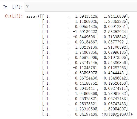
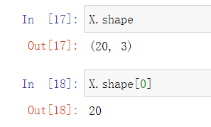
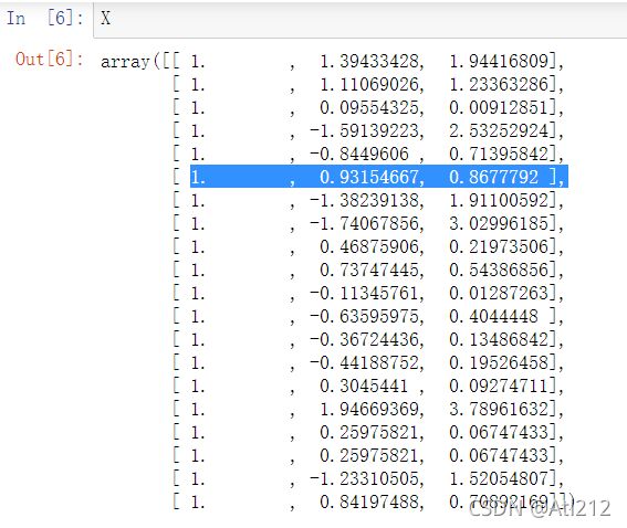
NumPy(NumericalPython)是Python中最基础、最重要的科学计算库之一,提供了高性能的多维数组(ndarray)对象和大量数学函数,是许多数据科学、机器学习库(如Pandas、SciPy、TensorFlow等)的基础依赖。1.创建一个numpy里面的一维数组importnumpyasnp###通过array方法创建一个ndarrayarray1=np.array([1,2,3
- 深度学习篇---昇腾NPU&CANN 工具包
Atticus-Orion
上位机知识篇图像处理篇深度学习篇深度学习人工智能NPU昇腾CANN
介绍昇腾NPU是华为推出的神经网络处理器,具有强大的AI计算能力,而CANN工具包则是面向AI场景的异构计算架构,用于发挥昇腾NPU的性能优势。以下是详细介绍:昇腾NPU架构设计:采用达芬奇架构,是一个片上系统,主要由特制的计算单元、大容量的存储单元和相应的控制单元组成。集成了多个CPU核心,包括控制CPU和AICPU,前者用于控制处理器整体运行,后者承担非矩阵类复杂计算。此外,还拥有AICore
- 深度学习图像分类数据集—桃子识别分类
AI街潜水的八角
深度学习图像数据集深度学习分类人工智能
该数据集为图像分类数据集,适用于ResNet、VGG等卷积神经网络,SENet、CBAM等注意力机制相关算法,VisionTransformer等Transformer相关算法。数据集信息介绍:桃子识别分类:['B1','M2','R0','S3']训练数据集总共有6637张图片,每个文件夹单独放一种数据各子文件夹图片统计:·B1:1601张图片·M2:1800张图片·R0:1601张图片·S3:
- 使用NVIDIA NeRF将2D图像转换为逼真的3D模型(Python)
ByteWhiz
3dpython计算机视觉Python
使用NVIDIANeRF将2D图像转换为逼真的3D模型(Python)NeuralRadianceFields(NeRF)是一种强大的方法,可以将2D图像转换为逼真的3D模型。它使用神经网络来建模场景的辐射场,并通过渲染多个视角的图像来重建3D模型。在本文中,我们将使用Python和NVIDIANeRF库来实现这一过程。首先,我们需要安装所需的库。我们可以通过以下命令使用pip安装NVIDIANe
- 微算法科技的前沿探索:量子机器学习算法在视觉任务中的革新应用
MicroTech2025
量子计算算法
在信息技术飞速发展的今天,计算机视觉作为人工智能领域的重要分支,正逐步渗透到我们生活的方方面面。从自动驾驶到人脸识别,从医疗影像分析到安防监控,计算机视觉技术展现了巨大的应用潜力。然而,随着视觉任务复杂度的不断提升,传统机器学习算法在处理大规模、高维度数据时遇到了计算瓶颈。在此背景下,量子计算作为一种颠覆性的计算模式,以其独特的并行处理能力和指数级增长的计算空间,为解决这一难题提供了新的思路。微算
- NumPy-@运算符详解
GG不是gg
numpynumpy
NumPy-@运算符详解一、@运算符的起源与设计目标1.从数学到代码:符号的统一2.设计目标二、@运算符的核心语法与运算规则1.基础用法:二维矩阵乘法2.一维向量的矩阵语义3.高维数组:批次矩阵运算4.广播机制:灵活的形状匹配三、@运算符与其他乘法方式的核心区别1.对比`np.dot()`2.对比元素级乘法`*`3.对比`np.matrix`的`*`运算符四、典型应用场景:从基础到高阶1.深度学习
- NLP_知识图谱_大模型——个人学习记录
macken9999
自然语言处理知识图谱大模型自然语言处理知识图谱学习
1.自然语言处理、知识图谱、对话系统三大技术研究与应用https://github.com/lihanghang/NLP-Knowledge-Graph深度学习-自然语言处理(NLP)-知识图谱:知识图谱构建流程【本体构建、知识抽取(实体抽取、关系抽取、属性抽取)、知识表示、知识融合、知识存储】-元気森林-博客园https://www.cnblogs.com/-402/p/16529422.htm
- 解决 Python 包安装失败问题:以 accelerate 为例
在使用Python开发项目时,我们经常会遇到依赖包安装失败的问题。今天,我们就以accelerate包为例,详细探讨一下可能的原因以及解决方法。通过这篇文章,你将了解到Python包安装失败的常见原因、如何切换镜像源、如何手动安装包,以及一些实用的注意事项。一、问题背景在开发一个深度学习项目时,我需要安装accelerate包来优化模型的训练过程。然而,当我运行以下命令时:bash复制pipins
- 在mac m1基于llama.cpp运行deepseek
lama.cpp是一个高效的机器学习推理库,目标是在各种硬件上实现LLM推断,保持最小设置和最先进性能。llama.cpp支持1.5位、2位、3位、4位、5位、6位和8位整数量化,通过ARMNEON、Accelerate和Metal支持Apple芯片,使得在MACM1处理器上运行Deepseek大模型成为可能。1下载llama.cppgitclonehttps://github.com/ggerg
- 图神经网络:挖掘关系数据中的宝藏
图神经网络:挖掘关系数据中的宝藏在浩瀚的数据海洋中,蕴藏着一类特殊而强大的资源——关系数据。它们不是孤立的点,而是相互连接、彼此影响的复杂网络:社交平台上朋友的朋友、电商系统中商品与用户的互动、蛋白质分子内原子的结合、城市交通网中的道路连接……这些数据天然以图的形式存在,节点代表实体,边则承载着实体间千丝万缕的关系。传统的数据挖掘工具面对这些盘根错节的结构往往力不从心,而图神经网络(GNN)的崛起
- 从RNN循环神经网络到Transformer注意力机制:解析神经网络架构的华丽蜕变
熊猫钓鱼>_>
神经网络rnntransformer
1.引言在自然语言处理和序列建模领域,神经网络架构经历了显著的演变。从早期的循环神经网络(RNN)到现代的Transformer架构,这一演变代表了深度学习方法在处理序列数据方面的重大进步。本文将深入比较这两种架构,分析它们的工作原理、优缺点,并通过实验结果展示它们在实际应用中的性能差异。2.循环神经网络(RNN)2.1基本原理循环神经网络是专门为处理序列数据而设计的神经网络架构。RNN的核心思想
- 【机器学习笔记Ⅰ】9 特征缩放
巴伦是只猫
机器学习机器学习笔记人工智能
特征缩放(FeatureScaling)详解特征缩放是机器学习数据预处理的关键步骤,旨在将不同特征的数值范围统一到相近的尺度,从而加速模型训练、提升性能并避免某些特征主导模型。1.为什么需要特征缩放?(1)问题背景量纲不一致:例如:特征1:年龄(范围0-100)特征2:收入(范围0-1,000,000)梯度下降的困境:量纲大的特征(如收入)会导致梯度更新方向偏离最优路径,收敛缓慢。量纲小的特征(如
- 如何使用Python实现交通工具识别
如何使用Python实现交通工具识别文章目录技术架构功能流程识别逻辑用户界面增强特性依赖项主要类别内容展示该系统是一个基于深度学习的交通工具识别工具,具备以下核心功能与特点:技术架构使用预训练的ResNet50卷积神经网络模型(来自ImageNet数据集)集成图像增强预处理技术(随机裁剪、旋转、翻转等)采用多数投票机制提升预测稳定性基于置信度评分的结果筛选策略功能流程用户通过GUI界面选择待识别图
- 【EGSR2025】材质+扩散模型+神经网络相关论文整理随笔(四)
Superstarimage
文献随笔材质神经网络人工智能扩散模型
AnevaluationofSVBRDFPredictionfromGenerativeImageModelsforAppearanceModelingof3DScenes输入3D场景的几何和一张参考图像,通过扩散模型和SVBRDF预测器获取多视角的材质maps,这些maps最终合并成场景的纹理地图集,并支持在任意视角、任意光照条件下进行重新渲染。样例图如下:在当前时代的技术背景下,生成与几何匹配
- Python OpenCV教程从入门到精通的全面指南【文末送书】
一键难忘
pythonopencv开发语言
文章目录PythonOpenCV从入门到精通1.安装OpenCV2.基本操作2.1读取和显示图像2.2图像基本操作3.图像处理3.1图像转换3.2图像阈值处理3.3图像平滑4.边缘检测和轮廓4.1Canny边缘检测4.2轮廓检测5.高级操作5.1特征检测5.2目标跟踪5.3深度学习与OpenCVPythonOpenCV从入门到精通【文末送书】PythonOpenCV从入门到精通OpenCV(Ope
- CNN 猫狗识别:从理论到实战的深度解析
爱熬夜的小古
cnn深度学习人工智能
在计算机视觉领域,卷积神经网络(ConvolutionalNeuralNetwork,CNN)凭借其强大的特征提取和模式识别能力,成为图像分类任务的主流技术。猫狗识别作为经典的图像分类问题,不仅能帮助我们理解CNN的工作原理,还能为实际应用提供技术支持。本文将深入探讨CNN在猫狗识别中的应用,从理论基础到实战代码,带你全面掌握这项技术。一、CNN基础理论概述(一)CNN的核心组件卷积层:是CNN的
- 第八周 tensorflow实现猫狗识别
降花绘
365天深度学习tensorflow系列tensorflow深度学习人工智能
本文为365天深度学习训练营内部限免文章(版权归K同学啊所有)**参考文章地址:[TensorFlow入门实战|365天深度学习训练营-第8周:猫狗识别(训练营内部成员可读)]**作者:K同学啊文章目录一、本周学习内容:1、自己搭建VGG16网络2、了解model.train_on_batch()3、了解tqdm,并使用tqdm实现可视化进度条二、前言三、电脑环境四、前期准备1、导入相关依赖项2、
- 深度学习实战-使用TensorFlow与Keras构建智能模型
程序员Gloria
Python超入门TensorFlowpython
深度学习实战-使用TensorFlow与Keras构建智能模型深度学习已经成为现代人工智能的重要组成部分,而Python则是实现深度学习的主要编程语言之一。本文将探讨如何使用TensorFlow和Keras构建深度学习模型,包括必要的代码实例和详细的解析。1.深度学习简介深度学习是机器学习的一个分支,使用多层神经网络来学习和表示数据中的复杂模式。其广泛应用于图像识别、自然语言处理、推荐系统等领域。
- AI在垂直领域的深度应用:医疗、金融与自动驾驶的革新之路
AI在垂直领域的深度应用:医疗、金融与自动驾驶的革新之路一、医疗领域:AI驱动的精准诊疗与效率提升1.医学影像诊断AI算法通过深度学习技术,已实现对X光、CT、MRI等影像的快速分析,辅助医生检测癌症、骨折等疾病。例如,GoogleDeepMind的AI系统在乳腺癌筛查中,误检率比人类专家低9.4%;中国的推想医疗AI系统可在20秒内完成肺部CT扫描分析,为急诊救治争取黄金时间。2.药物研发传统药
- 专题:2025云计算与AI技术研究趋势报告|附200+份报告PDF、原数据表汇总下载
原文链接:https://tecdat.cn/?p=42935关键词:2025,云计算,AI技术,市场趋势,深度学习,公有云,研究报告云计算和AI技术正以肉眼可见的速度重塑商业世界。过去十年,全球云服务收入激增8倍,中国云计算市场规模突破6000亿元,而深度学习算法的应用量更是暴涨400倍。这些数字背后,是企业从“自建机房”到“云原生开发”的转型,是AI从“实验室”走向“产业级应用”的跨越。本报告
- 【大模型与机器学习解惑】什么是A/B测试,为何进行A/B测试?
以下内容将围绕机器学习中的A/B测试展开,从概念与背景到实施细节、示例代码、优化思路和未来建议,并在最后给出一个整体的“输出目录”供参考。目录什么是机器学习的A/B测试为何要进行A/B测试A/B测试的实施流程示例代码与详细解释优化方向与未来建议结语1.什么是机器学习的A/B测试A/B测试(也常被称作对照试验、SplitTest)最早多用于互联网产品的功能或界面迭代中,指的是将用户或样本随机分为两组
- 【深度学习解惑】在实践中如何发现和修正RNN训练过程中的数值不稳定?
云博士的AI课堂
大模型技术开发与实践哈佛博后带你玩转机器学习深度学习深度学习rnn人工智能tensorflowpytorch神经网络机器学习
在实践中发现和修正RNN训练过程中的数值不稳定目录引言与背景介绍原理解释代码说明与实现应用场景与案例分析实验设计与结果分析性能分析与技术对比常见问题与解决方案创新性与差异性说明局限性与挑战未来建议和进一步研究扩展阅读与资源推荐图示与交互性内容语言风格与通俗化表达互动交流1.引言与背景介绍循环神经网络(RNN)在处理序列数据时表现出色,但训练过程中常面临梯度消失和梯度爆炸问题,导致数值不稳定。当网络
- 【深度学习实战】当前三个最佳图像分类模型的代码详解
云博士的AI课堂
大模型技术开发与实践哈佛博后带你玩转机器学习深度学习深度学习人工智能分类模型机器学习TransformerEfficientNetConvNeXt
下面给出三个在当前图像分类任务中精度表现突出的模型示例,分别基于SwinTransformer、EfficientNet与ConvNeXt。每个模型均包含:训练代码(使用PyTorch)从预训练权重开始微调(也可注释掉预训练选项,从头训练)数据集目录结构:└──dataset_root├──buy#第一类图像└──nobuy#第二类图像随机拆分:80%训练,20%验证每个Epoch输出一次loss
- 第35周—————糖尿病预测模型优化探索
目录目录前言1.检查GPU2.查看数据编辑3.划分数据集4.创建模型与编译训练5.编译及训练模型6.结果可视化7.总结前言本文为365天深度学习训练营中的学习记录博客原作者:K同学啊1.检查GPUimporttorch.nnasnnimporttorch.nn.functionalasFimporttorchvision,torch#设置硬件设备,如果有GPU则使用,没有则使用cpudevice=
- 《从依赖纠缠到接口协作:ASP.NET Core注入式开发指南》
后端
在C#的ASP.NETCore开发中,依赖注入绝非简单的技术技巧,而是重构代码关系的底层逻辑。它像一套隐形的神经网络,让程序模块摆脱硬编码的束缚,在运行时实现动态连接,从而为系统注入可测试、可进化的核心生命力。理解其深层价值,需要穿透"服务注册与获取"的表层操作,触及它对软件设计哲学的重塑。依赖注入的本质,是对"依赖关系"的去中心化治理。传统开发中,模块间的依赖如同藤蔓缠绕的树木,一个组件直接创建
- 详解LLMOps,将DevOps用于大语言模型开发
大家好,在机器学习领域,随着技术的不断发展,将大型语言模型(LLMs)集成到商业产品中已成为一种趋势,同时也带来了许多挑战。为了有效应对这些挑战,数据科学家们转向了一种新型的DevOps实践LLM-OPS,专为大型语言模型的开发和维护而设计。本文将介绍LLM-OPS的核心思想,并分析这一策略如何帮助数据科学家更高效地运用DevOps的优秀实践,从而在语言模型的开发和部署过程中,提升工作效率和成果的
- java线程Thread和Runnable区别和联系
zx_code
javajvmthread多线程Runnable
我们都晓得java实现线程2种方式,一个是继承Thread,另一个是实现Runnable。
模拟窗口买票,第一例子继承thread,代码如下
package thread;
public class ThreadTest {
public static void main(String[] args) {
Thread1 t1 = new Thread1(
- 【转】JSON与XML的区别比较
丁_新
jsonxml
1.定义介绍
(1).XML定义
扩展标记语言 (Extensible Markup Language, XML) ,用于标记电子文件使其具有结构性的标记语言,可以用来标记数据、定义数据类型,是一种允许用户对自己的标记语言进行定义的源语言。 XML使用DTD(document type definition)文档类型定义来组织数据;格式统一,跨平台和语言,早已成为业界公认的标准。
XML是标
- c++ 实现五种基础的排序算法
CrazyMizzz
C++c算法
#include<iostream>
using namespace std;
//辅助函数,交换两数之值
template<class T>
void mySwap(T &x, T &y){
T temp = x;
x = y;
y = temp;
}
const int size = 10;
//一、用直接插入排
- 我的软件
麦田的设计者
我的软件音乐类娱乐放松
这是我写的一款app软件,耗时三个月,是一个根据央视节目开门大吉改变的,提供音调,猜歌曲名。1、手机拥有者在android手机市场下载本APP,同意权限,安装到手机上。2、游客初次进入时会有引导页面提醒用户注册。(同时软件自动播放背景音乐)。3、用户登录到主页后,会有五个模块。a、点击不胫而走,用户得到开门大吉首页部分新闻,点击进入有新闻详情。b、
- linux awk命令详解
被触发
linux awk
awk是行处理器: 相比较屏幕处理的优点,在处理庞大文件时不会出现内存溢出或是处理缓慢的问题,通常用来格式化文本信息
awk处理过程: 依次对每一行进行处理,然后输出
awk命令形式:
awk [-F|-f|-v] ‘BEGIN{} //{command1; command2} END{}’ file
[-F|-f|-v]大参数,-F指定分隔符,-f调用脚本,-v定义变量 var=val
- 各种语言比较
_wy_
编程语言
Java Ruby PHP 擅长领域
- oracle 中数据类型为clob的编辑
知了ing
oracle clob
public void updateKpiStatus(String kpiStatus,String taskId){
Connection dbc=null;
Statement stmt=null;
PreparedStatement ps=null;
try {
dbc = new DBConn().getNewConnection();
//stmt = db
- 分布式服务框架 Zookeeper -- 管理分布式环境中的数据
矮蛋蛋
zookeeper
原文地址:
http://www.ibm.com/developerworks/cn/opensource/os-cn-zookeeper/
安装和配置详解
本文介绍的 Zookeeper 是以 3.2.2 这个稳定版本为基础,最新的版本可以通过官网 http://hadoop.apache.org/zookeeper/来获取,Zookeeper 的安装非常简单,下面将从单机模式和集群模式两
- tomcat数据源
alafqq
tomcat
数据库
JNDI(Java Naming and Directory Interface,Java命名和目录接口)是一组在Java应用中访问命名和目录服务的API。
没有使用JNDI时我用要这样连接数据库:
03. Class.forName("com.mysql.jdbc.Driver");
04. conn
- 遍历的方法
百合不是茶
遍历
遍历
在java的泛
- linux查看硬件信息的命令
bijian1013
linux
linux查看硬件信息的命令
一.查看CPU:
cat /proc/cpuinfo
二.查看内存:
free
三.查看硬盘:
df
linux下查看硬件信息
1、lspci 列出所有PCI 设备;
lspci - list all PCI devices:列出机器中的PCI设备(声卡、显卡、Modem、网卡、USB、主板集成设备也能
- java常见的ClassNotFoundException
bijian1013
java
1.java.lang.ClassNotFoundException: org.apache.commons.logging.LogFactory 添加包common-logging.jar2.java.lang.ClassNotFoundException: javax.transaction.Synchronization
- 【Gson五】日期对象的序列化和反序列化
bit1129
反序列化
对日期类型的数据进行序列化和反序列化时,需要考虑如下问题:
1. 序列化时,Date对象序列化的字符串日期格式如何
2. 反序列化时,把日期字符串序列化为Date对象,也需要考虑日期格式问题
3. Date A -> str -> Date B,A和B对象是否equals
默认序列化和反序列化
import com
- 【Spark八十六】Spark Streaming之DStream vs. InputDStream
bit1129
Stream
1. DStream的类说明文档:
/**
* A Discretized Stream (DStream), the basic abstraction in Spark Streaming, is a continuous
* sequence of RDDs (of the same type) representing a continuous st
- 通过nginx获取header信息
ronin47
nginx header
1. 提取整个的Cookies内容到一个变量,然后可以在需要时引用,比如记录到日志里面,
if ( $http_cookie ~* "(.*)$") {
set $all_cookie $1;
}
变量$all_cookie就获得了cookie的值,可以用于运算了
- java-65.输入数字n,按顺序输出从1最大的n位10进制数。比如输入3,则输出1、2、3一直到最大的3位数即999
bylijinnan
java
参考了网上的http://blog.csdn.net/peasking_dd/article/details/6342984
写了个java版的:
public class Print_1_To_NDigit {
/**
* Q65.输入数字n,按顺序输出从1最大的n位10进制数。比如输入3,则输出1、2、3一直到最大的3位数即999
* 1.使用字符串
- Netty源码学习-ReplayingDecoder
bylijinnan
javanetty
ReplayingDecoder是FrameDecoder的子类,不熟悉FrameDecoder的,可以先看看
http://bylijinnan.iteye.com/blog/1982618
API说,ReplayingDecoder简化了操作,比如:
FrameDecoder在decode时,需要判断数据是否接收完全:
public class IntegerH
- js特殊字符过滤
cngolon
js特殊字符js特殊字符过滤
1.js中用正则表达式 过滤特殊字符, 校验所有输入域是否含有特殊符号function stripscript(s) { var pattern = new RegExp("[`~!@#$^&*()=|{}':;',\\[\\].<>/?~!@#¥……&*()——|{}【】‘;:”“'。,、?]"
- hibernate使用sql查询
ctrain
Hibernate
import java.util.Iterator;
import java.util.List;
import java.util.Map;
import org.hibernate.Hibernate;
import org.hibernate.SQLQuery;
import org.hibernate.Session;
import org.hibernate.Transa
- linux shell脚本中切换用户执行命令方法
daizj
linuxshell命令切换用户
经常在写shell脚本时,会碰到要以另外一个用户来执行相关命令,其方法简单记下:
1、执行单个命令:su - user -c "command"
如:下面命令是以test用户在/data目录下创建test123目录
[root@slave19 /data]# su - test -c "mkdir /data/test123"
- 好的代码里只要一个 return 语句
dcj3sjt126com
return
别再这样写了:public boolean foo() { if (true) { return true; } else { return false;
- Android动画效果学习
dcj3sjt126com
android
1、透明动画效果
方法一:代码实现
public View onCreateView(LayoutInflater inflater, ViewGroup container, Bundle savedInstanceState)
{
View rootView = inflater.inflate(R.layout.fragment_main, container, fals
- linux复习笔记之bash shell (4)管道命令
eksliang
linux管道命令汇总linux管道命令linux常用管道命令
转载请出自出处:
http://eksliang.iteye.com/blog/2105461
bash命令执行的完毕以后,通常这个命令都会有返回结果,怎么对这个返回的结果做一些操作呢?那就得用管道命令‘|’。
上面那段话,简单说了下管道命令的作用,那什么事管道命令呢?
答:非常的经典的一句话,记住了,何为管
- Android系统中自定义按键的短按、双击、长按事件
gqdy365
android
在项目中碰到这样的问题:
由于系统中的按键在底层做了重新定义或者新增了按键,此时需要在APP层对按键事件(keyevent)做分解处理,模拟Android系统做法,把keyevent分解成:
1、单击事件:就是普通key的单击;
2、双击事件:500ms内同一按键单击两次;
3、长按事件:同一按键长按超过1000ms(系统中长按事件为500ms);
4、组合按键:两个以上按键同时按住;
- asp.net获取站点根目录下子目录的名称
hvt
.netC#asp.nethovertreeWeb Forms
使用Visual Studio建立一个.aspx文件(Web Forms),例如hovertree.aspx,在页面上加入一个ListBox代码如下:
<asp:ListBox runat="server" ID="lbKeleyiFolder" />
那么在页面上显示根目录子文件夹的代码如下:
string[] m_sub
- Eclipse程序员要掌握的常用快捷键
justjavac
javaeclipse快捷键ide
判断一个人的编程水平,就看他用键盘多,还是鼠标多。用键盘一是为了输入代码(当然了,也包括注释),再有就是熟练使用快捷键。 曾有人在豆瓣评
《卓有成效的程序员》:“人有多大懒,才有多大闲”。之前我整理了一个
程序员图书列表,目的也就是通过读书,让程序员变懒。 写道 程序员作为特殊的群体,有的人可以这么懒,懒到事情都交给机器去做,而有的人又可
- c++编程随记
lx.asymmetric
C++笔记
为了字体更好看,改变了格式……
&&运算符:
#include<iostream>
using namespace std;
int main(){
int a=-1,b=4,k;
k=(++a<0)&&!(b--
- linux标准IO缓冲机制研究
音频数据
linux
一、什么是缓存I/O(Buffered I/O)缓存I/O又被称作标准I/O,大多数文件系统默认I/O操作都是缓存I/O。在Linux的缓存I/O机制中,操作系统会将I/O的数据缓存在文件系统的页缓存(page cache)中,也就是说,数据会先被拷贝到操作系统内核的缓冲区中,然后才会从操作系统内核的缓冲区拷贝到应用程序的地址空间。1.缓存I/O有以下优点:A.缓存I/O使用了操作系统内核缓冲区,
- 随想 生活
暗黑小菠萝
生活
其实账户之前就申请了,但是决定要自己更新一些东西看也是最近。从毕业到现在已经一年了。没有进步是假的,但是有多大的进步可能只有我自己知道。
毕业的时候班里12个女生,真正最后做到软件开发的只要两个包括我,PS:我不是说测试不好。当时因为考研完全放弃找工作,考研失败,我想这只是我的借口。那个时候才想到为什么大学的时候不能好好的学习技术,增强自己的实战能力,以至于后来找工作比较费劲。我
- 我认为POJO是一个错误的概念
windshome
javaPOJO编程J2EE设计
这篇内容其实没有经过太多的深思熟虑,只是个人一时的感觉。从个人风格上来讲,我倾向简单质朴的设计开发理念;从方法论上,我更加倾向自顶向下的设计;从做事情的目标上来看,我追求质量优先,更愿意使用较为保守和稳妥的理念和方法。
&