关于神经网络模型及搭建基础的神经网络
目录
关于神经网络模型
神经网络模型
正向、反向传播公式
搭建网络
搭建网络的一般步骤
具体实现
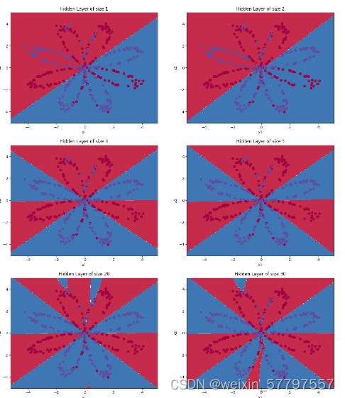
实验结果
关于神经网络模型
神经网络模型建立在很多神经元之上,每一个神经元又是一个个学习模型。这些神经元(也叫激活单元,activation unit)采纳一些特征作为输出,并且根据本身的模型提供一个输出。
-
神经网络模型
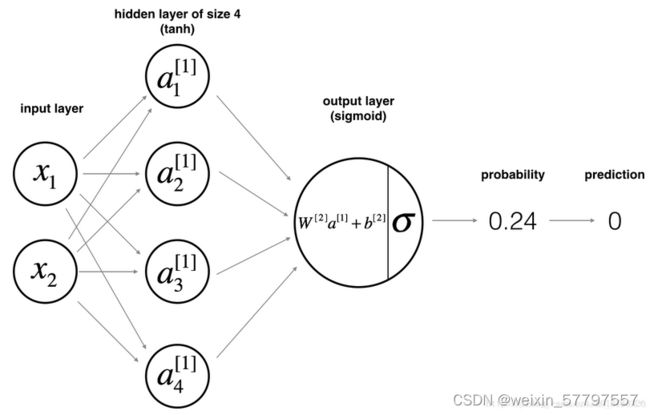
- 输入层:输入特征 x 1 、 x 2 它们被竖直地堆叠起来, 包含了神经网络的输入
- 隐藏层:四个结点, 在一个神经网络中,当你使用监督学习训练它的时候,训练集包含了输入 x也包含了目标输出 y,所以术语隐藏层的含义是在训练集中,这些中间结点的准确值我们是不知道到的,能看见输入的值,你也能看见输出的值,但是隐藏层中的东西,在训练集中你是无法看到的
- 输出层: 最后一层只由一个结点构成 , 这个只有一个结点的层被称为输出层
-
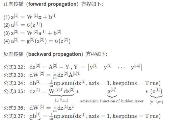
正向、反向传播公式
搭建网络
本实验目标是搭建一个有单隐藏层的二分类神经网络
搭建网络的一般步骤
1.定义网络结构(输入数量、隐藏单元数量)
2.初始化模型参数
3.循环:前向传播、计算损失、向后传播、梯度下降更新参数
具体实现
- 导入需要用的包,
matplotlib是用于绘图的库,planar_utils提供了在这个任务中使用的各种有用的功能
import numpy as np
import matplotlib.pyplot as plt
from planar_utils import plot_decision_boundary, sigmoid, load_planar_dataset- 整合为一个类,
np.random.randn(a,b)* 0.01来随机初始化一个维度为(a,b)的矩阵
class MyNet:
    parameters = {}
    cache = {}
    grads = {}
    cost = 0.0

    def __init__(self, X, Y, n_h):
        np.random.seed(2)
        W1 = np.random.randn(n_h, X.shape[0]) * 0.01
        b1 = np.zeros(shape=(n_h, 1))
        W2 = np.random.randn(Y.shape[0], n_h) * 0.01
        b2 = np.zeros(shape=(Y.shape[0], 1))
        self.parameters = {"W1": W1, "b1": b1, "W2": W2, "b2": b2}

#  W1 - 权重矩阵,维度为(n_h,n_x)
#  b1 - 偏向量,维度为(n_h,1)
#  W2 - 权重矩阵,维度为(n_y,n_h)
# b2 - 偏向量,维度为(n_y,1)- 向前传播
    def forward_propagation(self, X):
        W1 = self.parameters["W1"]
        b1 = self.parameters["b1"]
        W2 = self.parameters["W2"]
        b2 = self.parameters["b2"]
        Z1 = np.dot(W1, X) + b1
        A1 = np.tanh(Z1)
        Z2 = np.dot(W2, A1) + b2
        A2 = sigmoid(Z2)
        assert (A2.shape == (1, X.shape[1]))  # 断言确保数据格式是对的
        self.cache = {"Z1": Z1, "A1": A1, "Z2": Z2, "A2": A2}
return self.cache- 计算成本函数
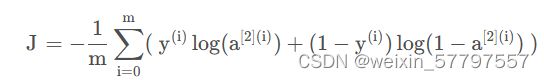
 def compute_cost(self, Y):
        m = Y.shape[1]
        # 计算成本
        logprobs = np.multiply(np.log(self.cache["A2"]), Y) + np.multiply((1 - Y), np.log(1 - self.cache["A2"]))
        self.cost = -np.sum(logprobs) / m
        self.cost = float(np.squeeze(self.cost))
        assert (isinstance(self.cost, float))
return self.cost- 反向传播
    def backward_propagation(self, X, Y):
        m = X.shape[1]
        W1 = self.parameters["W1"]
        W2 = self.parameters["W2"]
        A1 = self.cache["A1"]
        A2 = self.cache["A2"]

        dZ2 = A2 - Y
        dW2 = (1 / m) * np.dot(dZ2, A1.T)
        db2 = (1 / m) * np.sum(dZ2, axis=1, keepdims=True)
        dZ1 = np.multiply(np.dot(W2.T, dZ2), 1 - np.power(A1, 2))
        dW1 = (1 / m) * np.dot(dZ1, X.T)
        db1 = (1 / m) * np.sum(dZ1, axis=1, keepdims=True)
        self.grads = {"dW1": dW1, "db1": db1, "dW2": dW2, "db2": db2}
return self.grads- 更新参数,需要使用(dW1, db1, dW2, db2)来更新(W1, b1, W2, b2)
    def update_parameters(self, learning_rate=1.2):
        W1, W2 = self.parameters["W1"], self.parameters["W2"]
        b1, b2 = self.parameters["b1"], self.parameters["b2"]
        dW1, dW2 = self.grads["dW1"], self.grads["dW2"]
        db1, db2 = self.grads["db1"], self.grads["db2"]
        W1 = W1 - learning_rate * dW1
        b1 = b1 - learning_rate * db1
        W2 = W2 - learning_rate * dW2
        b2 = b2 - learning_rate * db2
        self.parameters = {"W1": W1, "b1": b1, "W2": W2, "b2": b2}
        return self.parameters

    def predict(self, X):
        self.cache = self.forward_propagation(X)
        predictions = np.round(self.cache["A2"])
return predictions- 训练模型
def nn_m(X, Y, net, num_iterations=10000, print_cost=True):
for i in range(num_iterations):
net.cache = net.forward_propagation(X)
net.cost = net.compute_cost(Y)
net.grads = net.backward_propagation(X, Y)
net.parameters = net.update_parameters(learning_rate=1.2)
if print_cost:
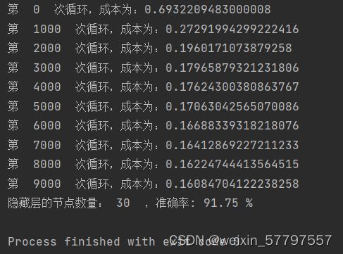
if i % 1000 == 0:
print("第 ", i, " 次循环,成本为:" + str(net.cost))
if __name__ == '__main__':
X, Y = load_planar_dataset()
plt.figure(figsize=(16, 32))
hidden_layer_sizes = [1, 2, 4, 5, 20, 30] # 隐藏层结点数量
for i, n_h in enumerate(hidden_layer_sizes):
net = MyNet(X, Y, n_h)
plt.subplot(5, 2, i+1)
plt.title('Hidden Layer of size %d' % n_h)
nn_m(X, Y, net)
plot_decision_boundary(lambda x: net.predict(x.T), X, Y)
y_pre = net.predict(X)
accuracy = float((np.dot(Y, y_pre.T) + np.dot(1 - Y, 1 - y_pre.T)) / float(Y.size) * 100)
print("隐藏层的节点数量: {} ,准确率: {} %".format(n_h, accuracy))
plt.show()实验结果
数据集及完整代码:https://blog.csdn.net/weixin_36815313/article/details/105342898