Python吴恩达深度学习作业8 -- 深度神经网络的梯度检验
梯度检验
假设你是致力于在全球范围内提供移动支付的团队的一员,被上级要求建立深度学习模型来检测欺诈行为–每当有人进行支付时,你都应该确认该支付是否可能是欺诈性的,例如用户的账户已被黑客入侵。
但是模型的反向传播很难实现,有时还会有错误。因为这是关键的应用任务,所以你公司的CEO要反复确定反向传播的实现是正确的。CEO要求你证明你的反向传播实际上是有效的!为了保证这一点,你将应用到"梯度检验"。
import numpy as np
from testCases import *
from gc_utils import sigmoid, relu, dictionary_to_vector, vector_to_dictionary, gradients_to_vector
1 梯度检验原理
反向传播计算梯度 ∂ J ∂ θ \frac {\partial J}{\partial \theta} ∂θ∂J,其中 θ \theta θ表示模型的参数。使用正向传播和损失函数来计算 J J J。
由于正向传播相对容易实现,相信你有信心做到这一点,确定100%计算正确的损失 J J J。为此,你可以使用 J J J来验证代码 ∂ J ∂ θ \frac {\partial J}{\partial \theta} ∂θ∂J。
让我们回顾一下导师(或者说梯度)的定义:
∂ J ∂ θ = lim ε → 0 J ( θ + ε ) − J ( θ − ε ) 2 ε (1) \frac{\partial J}{\partial \theta} = \lim_{\varepsilon \to 0} \frac{J(\theta + \varepsilon) - J(\theta - \varepsilon)}{2 \varepsilon} \tag{1} ∂θ∂J=ε→0lim2εJ(θ+ε)−J(θ−ε)(1)
如果你还不熟悉" lim ε → 0 \displaystyle \lim_{\varepsilon \to 0} ε→0lim“表示法,其意思只是"当 ε \varepsilon ε值取向很小时”。
我们知道以下内容:
- ∂ J ∂ θ \frac {\partial J}{\partial \theta} ∂θ∂J是你要确保计算正确的对象。
- 你可以计算 J ( θ + ε ) J(\theta + \varepsilon) J(θ+ε)和 J ( θ − ε ) J(\theta - \varepsilon) J(θ−ε)(在 θ \theta θ是实数的情况下),因为要保证 J J J的实现是正确的。
2 一维梯度检查
思考一维线性函数 J ( θ ) = θ x J(\theta)=\theta x J(θ)=θx,该模型仅包含一个实数值参数 θ \theta θ,并以 x x x作为输入。
你将实现代码以计算 J ( . ) J(.) J(.)及其派生 ∂ J ∂ θ \frac {\partial J}{\partial \theta} ∂θ∂J,然后,你将使用梯度检验来确保 J J J的导数计算正确。
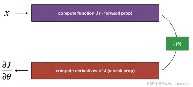
上图显示了关键的计算步骤:首先从 x x x开始,再评估函数 J ( x ) J(x) J(x)(正向传播),然后计算导数 ∂ J ∂ θ \frac {\partial J}{\partial \theta} ∂θ∂J(反向传播)。
练习:为此简单函数实现"正向传播"和"反向传播"。即在两个单独的函数中,计算 J ( . ) J(.) J(.)(正向传播)及相对于 θ \theta θ(反向传播)的导数。
def forward_propagation(x, theta):
    J = theta * x

    return J
x, theta = 2, 4
J = forward_propagation(x, theta)
print ("J = " + str(J))
J = 8
练习:现在,执行的反向传播步骤(导数计算)。也就是说,计算 J ( θ ) = θ x J(\theta)=\theta x J(θ)=θx相对于 θ \theta θ的导数。为避免进行演算,你应该得到 d θ = ∂ J ∂ θ = x d\theta = \frac {\partial J}{\partial \theta} = x dθ=∂θ∂J=x。
def backward_propagation(x, theta):
    dtheta = x
    return dtheta
x, theta = 2, 4
dtheta = backward_propagation(x, theta)
print ("dtheta = " + str(dtheta))
dtheta = 2
练习:为了展示backward_propagation()函数正确计算了梯度 ∂ J ∂ θ \frac {\partial J}{\partial \theta} ∂θ∂J,让我们实施梯度检验。
说明:
- 首先使用上式(1)和 ε \varepsilon ε的极小值计算“gradapprox”。以下是要遵循的步骤:
- θ + = θ + ε \theta^{+} = \theta + \varepsilon θ+=θ+ε
- θ − = θ − ε \theta^{-} = \theta - \varepsilon θ−=θ−ε
- J + = J ( θ + ) J^{+} = J(\theta^{+}) J+=J(θ+)
- J − = J ( θ − ) J^{-} = J(\theta^{-}) J−=J(θ−)
- g r a d a p p r o x = J + − J − 2 ε gradapprox = \frac{J^{+} - J^{-}}{2 \varepsilon} gradapprox=2εJ+−J−
- 然后使用反向传播计算梯度,并将结果存储在变量“grad”中
- 最后,使用以下公式计算“gradapprox”和“grad”之间的相对差:
d i f f e r e n c e = ∣ ∣ g r a d − g r a d a p p r o x ∣ ∣ 2 ∣ ∣ g r a d ∣ ∣ 2 + ∣ ∣ g r a d a p p r o x ∣ ∣ 2 (2) difference = \frac {\mid\mid grad - gradapprox \mid\mid_2}{\mid\mid grad \mid\mid_2 + \mid\mid gradapprox \mid\mid_2} \tag{2} difference=∣∣grad∣∣2+∣∣gradapprox∣∣2∣∣grad−gradapprox∣∣2(2)
你需要3个步骤来计算此公式:- 1.使用np.linalg.norm(…)计算分子
- 2.计算分母,调用np.linalg.norm(…)两次
- 3.相除
- 如果差异很小(例如小于 1 0 − 7 10^{-7} 10−7),则可以确信正确计算了梯度。否则,梯度计算可能会出错。
def gradient_check(x, theta, epsilon = 1e-7):
    # 用公式(1)的左边计算gradapprox。足够小,你不需要担心极限。
    thetaplus = theta + epsilon
    thetaminus = theta - epsilon
    J_plus = forward_propagation(x, thetaplus)
    J_minus = forward_propagation(x, thetaminus)
    gradapprox = (J_plus - J_minus) / (2 * epsilon)

    # 检查gradapprox是否足够接近backward_propagation()的输出
    grad = backward_propagation(x, theta)

    numerator = np.linalg.norm(grad - gradapprox)
    denominator = np.linalg.norm(grad) + np.linalg.norm(gradapprox)
    difference = numerator / denominator

    if difference < 1e-7:
        print ("The gradient is correct!")
    else:
        print ("The gradient is wrong!")

    return difference
x, theta = 2, 4
difference = gradient_check(x, theta)
print("difference = " + str(difference))
The gradient is correct!
difference = 2.919335883291695e-10
Nice!差异小于阈值 1 0 − 7 10^{-7} 10−7。因此可以放心,你已经在backward_propagation()中正确计算了梯度。
现在,在更一般的情况下,你的损失函数 J J J具有多个单个1D输入。当你训练神经网络时, θ \theta θ实际上由多个矩阵 W [ l ] W^{[l]} W[l]组成,并加上偏差 b l b^{l} bl!重要的是要知道如何对高维输入进行梯度检验。
3 N维梯度检验
下面描述了欺诈检测模型的正向传播和反向传播:
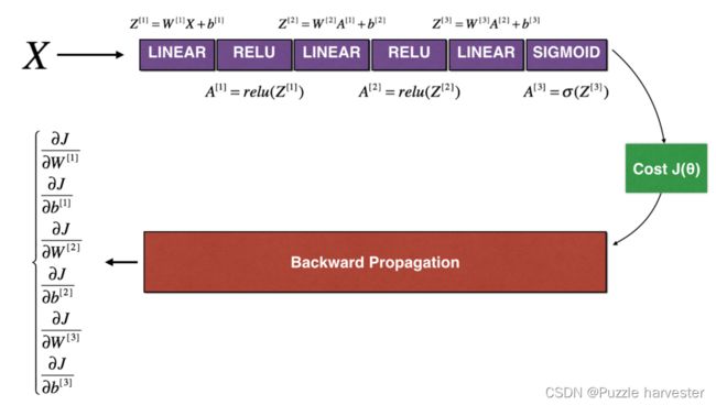
LINEAR -> RELU -> LINEAR -> RELU -> LINEAR -> SIGMOID
让我们看一下正向传播和反向传播的实现。
def forward_propagation_n(X, Y, parameters):

    # retrieve parameters
    m = X.shape[1]
    W1 = parameters["W1"]
    b1 = parameters["b1"]
    W2 = parameters["W2"]
    b2 = parameters["b2"]
    W3 = parameters["W3"]
    b3 = parameters["b3"]

    # LINEAR -> RELU -> LINEAR -> RELU -> LINEAR -> SIGMOID
    Z1 = np.dot(W1, X) + b1
    A1 = relu(Z1)
    Z2 = np.dot(W2, A1) + b2
    A2 = relu(Z2)
    Z3 = np.dot(W3, A2) + b3
    A3 = sigmoid(Z3)

    # Cost
    logprobs = np.multiply(-np.log(A3),Y) + np.multiply(-np.log(1 - A3), 1 - Y)
    cost = 1./m * np.sum(logprobs)

    cache = (Z1, A1, W1, b1, Z2, A2, W2, b2, Z3, A3, W3, b3)

    return cost, cache
现在,运行反向传播。
def backward_propagation_n(X, Y, cache):

    m = X.shape[1]
    (Z1, A1, W1, b1, Z2, A2, W2, b2, Z3, A3, W3, b3) = cache

    dZ3 = A3 - Y
    dW3 = 1./m * np.dot(dZ3, A2.T)
    db3 = 1./m * np.sum(dZ3, axis=1, keepdims = True)

    dA2 = np.dot(W3.T, dZ3)
    dZ2 = np.multiply(dA2, np.int64(A2 > 0))
    dW2 = 1./m * np.dot(dZ2, A1.T) * 2 # 去掉 *2
    db2 = 1./m * np.sum(dZ2, axis=1, keepdims = True)

    dA1 = np.dot(W2.T, dZ2)
    dZ1 = np.multiply(dA1, np.int64(A1 > 0))
    dW1 = 1./m * np.dot(dZ1, X.T)
    db1 = 4./m * np.sum(dZ1, axis=1, keepdims = True) # 4.改为1.

    gradients = {"dZ3": dZ3, "dW3": dW3, "db3": db3,
                 "dA2": dA2, "dZ2": dZ2, "dW2": dW2, "db2": db2,
                 "dA1": dA1, "dZ1": dZ1, "dW1": dW1, "db1": db1}

    return gradients
你在欺诈检测测试集上获得了初步的实验结果,但是这并不是100%确定的模型,毕竟没有东西是完美的!让我们实现梯度检验以验证你的梯度是否正确。
梯度检验原理
与1和2中一样,你想将“gradapprox”与通过反向传播计算的梯度进行比较。公式仍然是:
∂ J ∂ θ = lim ε → 0 J ( θ + ε ) − J ( θ − ε ) 2 ε (1) \frac{\partial J}{\partial \theta} = \lim_{\varepsilon \to 0} \frac{J(\theta + \varepsilon) - J(\theta - \varepsilon)}{2 \varepsilon} \tag{1} ∂θ∂J=ε→0lim2εJ(θ+ε)−J(θ−ε)(1)
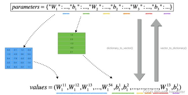
但是, θ \theta θ不再是标量。 而是一个叫做“参数”的字典。 我们为你实现了一个函数"dictionary_to_vector()"。它将“参数”字典转换为称为“值”的向量,该向量是通过将所有参数(W1, b1, W2, b2, W3, b3)重塑为向量并将它们串联而获得的。
反函数是“vector_to_dictionary”,它输出回“parameters”字典。
你将在 gradient_check_n()中用到这些函数
我们还使用gradients_to_vector()将“gradients”字典转换为向量“grad”。
练习:实现gradient_check_n()。
说明:这是伪代码,可帮助你实现梯度检验。
for each i in num_parameters:
- 计算
J_plus[i]:- 将 θ + \theta^{+} θ+设为
np.copy(parameters_values) - 将 θ + \theta^{+} θ+设为 θ i + + ε \theta_i^{+} + \varepsilon θi++ε
- 使用
forward_propagation_n(x, y, vector_to_dictionary(θ + \theta^+ θ+))计算 J i + J_i^+ Ji+
- 将 θ + \theta^{+} θ+设为
- 计算
J_minus [i]:也是用 θ − \theta^{-} θ− - 计算 g r a d a p p r o x [ i ] = J i + − J i − 2 ε gradapprox[i] = \frac{J^{+}_i - J^{-}_i}{2 \varepsilon} gradapprox[i]=2εJi+−Ji−
因此,你将获得向量gradapprox,其中gradapprox[i]是相对于parameter_values[i]的梯度的近似值。现在,你可以将此gradapprox向量与反向传播中的梯度向量进行比较。就像一维情况(步骤1’,2’,3’)一样计算:
d i f f e r e n c e = ∥ g r a d − g r a d a p p r o x ∥ 2 ∥ g r a d ∥ 2 + ∥ g r a d a p p r o x ∥ 2 (3) difference = \frac {\| grad - gradapprox \|_2}{\| grad \|_2 + \| gradapprox \|_2 } \tag{3} difference=∥grad∥2+∥gradapprox∥2∥grad−gradapprox∥2(3)
def gradient_check_n(parameters, gradients, X, Y, epsilon = 1e-7):

    # 设置变量
    parameters_values, _ = dictionary_to_vector(parameters)
    grad = gradients_to_vector(gradients)
    num_parameters = parameters_values.shape[0]
    J_plus = np.zeros((num_parameters, 1))
    J_minus = np.zeros((num_parameters, 1))
    gradapprox = np.zeros((num_parameters, 1))

    # 计算gradapprox
    for i in range(num_parameters):
        thetaplus = np.copy(parameters_values)
        thetaplus[i][0] = thetaplus[i][0] + epsilon
        J_plus[i], _ = forward_propagation_n(X, Y, vector_to_dictionary(thetaplus))

        thetaminus = np.copy(parameters_values)
        thetaminus[i][0] = thetaminus[i][0] - epsilon
        J_minus[i], _ =forward_propagation_n(X, Y, vector_to_dictionary(thetaminus))

        gradapprox[i] = (J_plus[i] - J_minus[i]) / (2. * epsilon)

    numerator = np.linalg.norm(grad - gradapprox)                                           # Step 1'
    denominator = np.linalg.norm(grad) + np.linalg.norm(gradapprox)                                         # Step 2'
    difference = numerator / denominator

    if difference > 1e-7:
        print ("There is a mistake in the backward propagation! difference = " + str(difference) )
    else:
        print ("Your backward propagation works perfectly fine! difference = " + str(difference) )

    return difference
X, Y, parameters = gradient_check_n_test_case()

cost, cache = forward_propagation_n(X, Y, parameters)
gradients = backward_propagation_n(X, Y, cache)
difference = gradient_check_n(parameters, gradients, X, Y)
There is a mistake in the backward propagation! difference = 0.2850931567761624
看起来backward_propagation_n代码似乎有错误!很好,你已经实现了梯度检验。返回到backward_propagation并尝试查找/更正错误(提示:检查dW2和db1)。如果你已解决问题,请重新运行梯度检验。请记住,如果修改代码,则需要重新执行定义backward_propagation_n()的单元格。
你可以进行梯度检验来证明你的导数计算的正确吗?即使作业的这一部分没有评分,我们也强烈建议你尝试查找错误并重新运行梯度检验,直到确信实现了正确的反向传播。
注意
- 梯度检验很慢!用 ∂ J ∂ θ ≈ J ( θ + ε ) − J ( θ − ε ) 2 ε \frac{\partial J}{\partial \theta} \approx \frac{J(\theta + \varepsilon) - J(\theta - \varepsilon)}{2 \varepsilon} ∂θ∂J≈2εJ(θ+ε)−J(θ−ε)逼近梯度在计算上是很耗费资源的。因此,我们不会在训练期间的每次迭代中都进行梯度检验。只需检查几次梯度是否正确。
- 至少如我们介绍的那样,梯度检验不适用于dropout。通常,你将运行不带dropout的梯度检验算法以确保你的backprop是正确的,然后添加dropout。
Nice!现在你可以确信你用于欺诈检测的深度学习模型可以正常工作!甚至可以用它来说服你的CEO。
你在此笔记本中应记住的内容:
- 梯度检验可验证反向传播的梯度与梯度的数值近似值之间的接近度(使用正向传播进行计算)。
- 梯度检验很慢,因此我们不会在每次训练中都运行它。通常,你仅需确保其代码正确即可运行它,然后将其关闭并将backprop用于实际的学习过程。
几次梯度是否正确。 - 至少如我们介绍的那样,梯度检验不适用于dropout。通常,你将运行不带dropout的梯度检验算法以确保你的backprop是正确的,然后添加dropout。
Nice!现在你可以确信你用于欺诈检测的深度学习模型可以正常工作!甚至可以用它来说服你的CEO。
你在此笔记本中应记住的内容:
- 梯度检验可验证反向传播的梯度与梯度的数值近似值之间的接近度(使用正向传播进行计算)。
- 梯度检验很慢,因此我们不会在每次训练中都运行它。通常,你仅需确保其代码正确即可运行它,然后将其关闭并将backprop用于实际的学习过程。