BlendMask实例分割模型热力图+可视化

---

提示：如果想实现其他实例分割模型，可以通过官方代码选择对应的配置文件。

---

前言

随着人工智能的不断发展，机器学习这门技术也越来越重要，很多人都开启了学习机器学习，本文就介绍了机器学习的基础内容。

---

提示：以下是本篇文章正文内容，下面案例可供参考

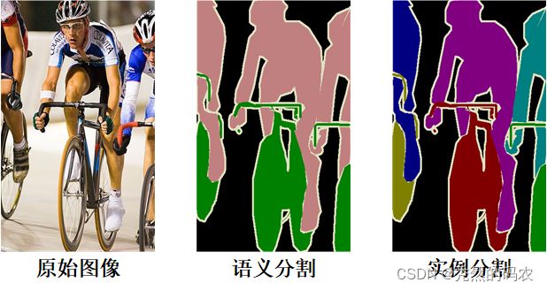
一、实例分割是什么？

话不多说，直接上图。

二、示例

这是代码的链接(Pytorch版本)
平台部署的直接百度，如果遇到解决不了的问题可以私信我。平台部署完后就可以直接上代码了。
目前平台支持的模型：BlendMask，BoxInst，CondInst，MEInst，SOLOv2等。

1.参数设置

模型选用的是BlendMask。
代码如下（示例）：

def get_parser():
    parser = argparse.ArgumentParser(description="Detectron2 Demo")
    parser.add_argument(
        "--config-file",
        default="D:/LIN/AdelaiDet-master/configs/BlendMask/R_50_1x.yaml",#配置参数文件
        metavar="FILE",
        help="path to config file",
    )
    parser.add_argument("--webcam", action="store_true", help="Take inputs from webcam.")
    parser.add_argument("--video-input", help="Path to video file.")
    parser.add_argument("--input",
                        default=["这里输入自己的待处理的图片路径"],
                        nargs="+", help="A list of space separated input images")
    parser.add_argument(
        "--output",
        help="A file or directory to save output visualizations. "
        "If not given, will show output in an OpenCV window.",
    )
    parser.add_argument(
        "--confidence-threshold",
        type=float,
        default=0.3,
        help="Minimum score for instance predictions to be shown",
    )
    parser.add_argument(
        "--opts",
        help="Modify config options using the command-line 'KEY VALUE' pairs",
        default=[],
        nargs=argparse.REMAINDER,
    )
    return parser

2.模型读入

这是模型加载的主函数内容，与官方代码一致。
代码如下（示例）：

if __name__ == "__main__":
    mp.set_start_method("spawn", force=True)
    args = get_parser().parse_args()
    logger = setup_logger()
    logger.info("Arguments: " + str(args))
    cfg = setup_cfg(args)
    demo = VisualizationDemo(cfg)

该处的cfg文件可以自己在其中修改超参数。

3.热力图

这是紧接着步骤2中的代码块，也就是模型配置加载完成后的操作(热力图)。
代码如下（示例）：

	args.input = glob.glob(os.path.expanduser(args.input[0]))
    for path in tqdm.tqdm(args.input, disable=not args.output):
            # use PIL, to be consistent with evaluation
            img = read_image(path, format="RGB")
         
    predictions, visualized_output = demo.run_on_image(img)
    x_visualize = visualized_output.get_image()[:, :, ::-1]
    # x_visualize = np.max((visualized_output.get_image()[:, :, ::-1]),axis=2) #返回每个通道的最大值
    h,w,c = x_visualize.shape
    x_visualize = abs((((x_visualize - np.min(x_visualize))/(np.max(x_visualize)-np.min(x_visualize)))*255).astype(np.uint8))#归一化并映射到0-255的整数，方便伪彩色化
    x_visualize = cv2.applyColorMap(x_visualize, cv2.COLORMAP_JET)  # 伪彩色处理COLORMAP_JET
    img_file = os.path.basename('33').split('.')[0]
    cv2.imwrite('D:/'+  img_file + '.jpg',x_visualize)

4.可视化

这是紧接着步骤2中的代码块，也就是模型配置加载完成后的操作(可视化)。
代码如下（示例）：

	if args.input:
        if os.path.isdir(args.input[0]):
            args.input = [os.path.join(args.input[0], fname) for fname in os.listdir(args.input[0])]
        elif len(args.input) == 1:
            args.input = glob.glob(os.path.expanduser(args.input[0]))
            assert args.input, "The input path(s) was not found"
        for path in tqdm.tqdm(args.input, disable=not args.output):
            # use PIL, to be consistent with evaluation
            img = read_image(path, format="BGR")
            start_time = time.time()
            predictions, visualized_output = demo.run_on_image(img)
            logger.info(
                "{}: detected {} instances in {:.2f}s".format(
                    path, len(predictions["instances"]), time.time() - start_time
                )
            )

            if args.output:
                if os.path.isdir(args.output):
                    assert os.path.isdir(args.output), args.output
                    out_filename = os.path.join(args.output, os.path.basename(path))
                else:
                    assert len(args.input) == 1, "Please specify a directory with args.output"
                    out_filename = args.output
                visualized_output.save(out_filename)
            else:
                cv2.imshow(WINDOW_NAME, visualized_output.get_image()[:, :, ::-1])
                img_file = os.path.basename('BlendMask').split('.')[0]
                cv2.imwrite('D:/'+ img_file + '.jpg',visualized_output.get_image()[:, :, ::-1]) #保存可视化图像
                

步骤3和步骤4互不影响，可择其一运行

---

总结

简单暴力，直接上图。
从左往右依次是原图，热力图和处理完后的图像可视化。

以上就是今天要讲的内容，本文仅仅简单介绍了一张图像可视化的实现流程，我们可以通过源码快速便捷地处理大批次的图像数据。