深度估计 ManyDepth 笔记

参考代码：manydepth
论文名称：The Temporal Opportunist: Self-Supervised Multi-Frame Monocular Depth

1. 概述

导读：这篇文章借鉴了多视图深度估计中的cost-volume方法（参考：cost-volume概念），并将其引入到单目的自监督深度估计网络中。这里将原来的双目图像换成了一对前后帧图像，从而去构建cost-volume克服之前的单目深度估计中的scale ambiguity问题。此外，为了克服单目情况下cost-volume的训练问题，文章提出了一系列的策略进行解决，如运动目标的滤除，从而极大提升了单目深度估计的性能。

笼统上看文章的方法是单目视觉与立体视觉的组合，其具有：

• 1）自监督的深度估计网络，在预测的时候可以输入一帧图像也可以输入多帧图像，自然多帧图像带来的效果更好；
• 2）对于图像中运动的目标和静止的场景往往会对深度估计网络带来影响，对此文章通过引入有效的损失函数与训练策略去解决了这个问题；
• 3）对于单目深度估计中scale ambiguity的问题，文章借鉴立体视觉中的cost-volume，利用单目的视频序列构建cost-volume；

文章的方法在单帧图像输入和多帧图像输入情况下进行深度估计的效果见下图所示：

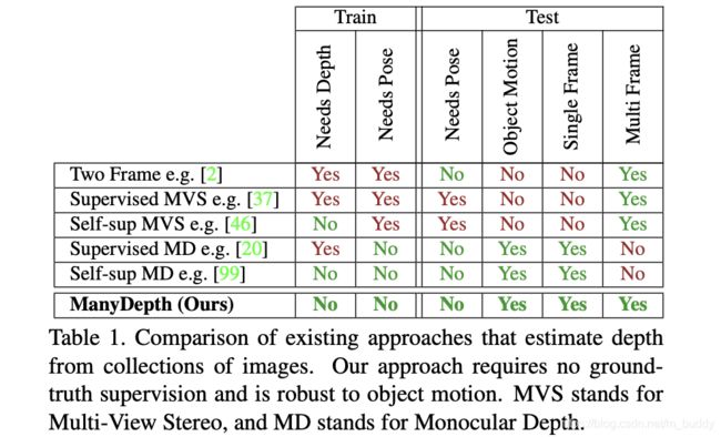
文章将深度估计中的一些方法在使用时需要的条件进行了分析，这些方法的要求为：

• 1）需要多帧图像作为输入；
• 2）相机不能静止；
• 3）深度估计训练时需要知道相机的位姿，甚至是测试时；
• 4）图像中没有移动的目标；

然后，将文章提出的方法与这些方法在使用限制上进行对比，见下表所示：

2. 方法设计

2.1 网络结构

文章的网络结构见下图所示：

从上图可以看到算法主要由：相机位姿估计网络，cost-volume构建，深度估计网络组成。

相机位姿估计网络：
这里使用相邻的两帧图像去估计相机的位姿$T_{t\to t+n},n\in \{-1,1\}$（文章中并没有使用未来帧，因而$n=-1$），则位姿被描述为：
$$T_{t\to t+n}={\theta }_{pose}(I_t,I_{t+n})$$

cost-volume构建：
cost-volume在文章算法中描述的是在不同深度下相邻帧像素上的差异，不过文章中并不是在图像的维度进行，而是在特征（stride=4）的维度上。按照最小深度和最大深度值：$d_{min},d_{max}$（文章中对于这两个超参数的设置是通过自适应的方式进行的，这个在后面的cost-volume部分进行说明）在$I_t$光轴的垂直方向上划分多个平面$\mathcal{P}$，之后在源图像的特征上使用计算得到的相机位姿信息和相机内参矩阵对特征进行变换得到$F_{t+n\to t,d},d\in \mathcal{P}$。之后cost-volume就是在变换后的源图像特征与目标图像特征上做绝对值差得到的。之后再与目标图像的特征组合起来经过解码器得到深度估计图。

深度估计网络:
这里深度估计的时候是使用了多帧的信息，因而深度估计部分被描述为：
$$D_t={\theta }_{depth}(I_t,I_{t-1},\dots ,I_{t-N})$$
也就是文章使用过往帧的数据作为输入去预测深度，代码中将其设置为$N=1$。之后在图像的维度上进行了重构误差监督，重构的过程描述为：
$$I_{t+n\to t}=I_{t+n}⟨proj(D_t,T_{t\to t+n},K)⟩$$
重构误差的计算与monodepth2的计算过程类似，描述为：
$$L_p=\underset{n}{\min }pe(I_t,I_{t+n\to t})$$
这里使用的重构损失为SSIM与L1范数的组合，也与monodepth2类似。

2.2 cost-volume机制

Adaptive cost-volume：
cost-volume的引入可以解决之前单目深度估计中scale ambiguity的问题，但是却因为实际的$d_{min},d_{max}$是未知的，对此文章引入了自适应的cost-volume机制。将$d_{min},d_{max}$通过在输入的数据中进行学习的方式得到，也就是网络通过训练的过程中自适应找到这两个参数（在batch预测的深度图$D_t$上进行统计，并在之后进行动量更新），之后在写checkpoint的时候一并写入，测试的时候取出使用。

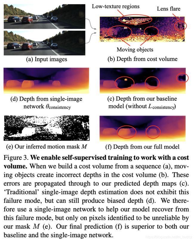
cost-volume中过拟合问题的处理：
一般意义上讲cost-volume机制的引入会使得结果更好，但是实际上还是会存在之前自监督方法的“孔洞”问题（这些区域存在目标的移动），见图c的b图。经过分析cost-volume中的信息只是在某些场合下是可信的，而在诸如目标移动/低纹理区域上是不置信的。而这些区域在图像的维度上进行重构的时候其重构的误差是很小的，因而这部分的cost-volume信息被过度信赖，需要一个mask将其排除，类似monodepth2中的auto-mask机制。这里由auto-mask产生的掩膜记为$M_A$。

在计算cost-volume的过程中，那些为0的区域就是需要被排除出去的区域，这里将其记为$M_c$。具体的cost-volume的计算过程描述为：

# manydepth/networks/resnet_encoder.py#157
def match_features(self, current_feats, lookup_feats, relative_poses, K, invK):
    """Compute a cost volume based on L1 difference between current_feats and lookup_feats.

    We backwards warp the lookup_feats into the current frame using the estimated relative
    pose, known intrinsics and using hypothesised depths self.warp_depths (which are either
    linear in depth or linear in inverse depth).

    If relative_pose == 0 then this indicates that the lookup frame is missing (i.e. we are
    at the start of a sequence), and so we skip it"""

    batch_cost_volume = []  # store all cost volumes of the batch
    cost_volume_masks = []  # store locations of '0's in cost volume for confidence

    for batch_idx in range(len(current_feats)):

        volume_shape = (self.num_depth_bins, self.matching_height, self.matching_width)
        cost_volume = torch.zeros(volume_shape, dtype=torch.float, device=current_feats.device)
        counts = torch.zeros(volume_shape, dtype=torch.float, device=current_feats.device)

        # select an item from batch of ref feats
        _lookup_feats = lookup_feats[batch_idx:batch_idx + 1]
        _lookup_poses = relative_poses[batch_idx:batch_idx + 1]

        _K = K[batch_idx:batch_idx + 1]
        _invK = invK[batch_idx:batch_idx + 1]
        world_points = self.backprojector(self.warp_depths, _invK)  # 将不同深度的平面从图像坐标映射到带有深度的相机坐标

        # loop through ref images adding to the current cost volume
        for lookup_idx in range(_lookup_feats.shape[1]):
            lookup_feat = _lookup_feats[:, lookup_idx]  # 1 x C x H x W
            lookup_pose = _lookup_poses[:, lookup_idx]

            # ignore missing images
            if lookup_pose.sum() == 0:
                continue

            lookup_feat = lookup_feat.repeat([self.num_depth_bins, 1, 1, 1])  # source图像特征处理，为了维度匹配
            pix_locs = self.projector(world_points, _K, lookup_pose)  # 相机坐标系经过变换到图像坐标（特征图维度）
            warped = F.grid_sample(lookup_feat, pix_locs, padding_mode='zeros', mode='bilinear',
                                   align_corners=True)  # 进行采样

            # mask values landing outside the image (and near the border)
            # we want to ignore edge pixels of the lookup images and the current image
            # because of zero padding in ResNet
            # Masking of ref image border
            x_vals = (pix_locs[..., 0].detach() / 2 + 0.5) * (
                self.matching_width - 1)  # convert from (-1, 1) to pixel values
            y_vals = (pix_locs[..., 1].detach() / 2 + 0.5) * (self.matching_height - 1)

            edge_mask = (x_vals >= 2.0) * (x_vals <= self.matching_width - 2) * \
                        (y_vals >= 2.0) * (y_vals <= self.matching_height - 2)
            edge_mask = edge_mask.float()

            # masking of current image
            current_mask = torch.zeros_like(edge_mask)
            current_mask[:, 2:-2, 2:-2] = 1.0
            edge_mask = edge_mask * current_mask  # 去除掉边界

            diffs = torch.abs(warped - current_feats[batch_idx:batch_idx + 1]).mean(
                1) * edge_mask  # 计算source特征经过不同深度平面映射之后与target特征的差距，cost-volume的关键

            # integrate into cost volume
            cost_volume = cost_volume + diffs
            counts = counts + (diffs > 0).float()
        # average over lookup images
        cost_volume = cost_volume / (counts + 1e-7)

        # if some missing values for a pixel location (i.e. some depths landed outside) then
        # set to max of existing values
        missing_val_mask = (cost_volume == 0).float()  # 未被匹配到的区域，"孔洞"区域
        if self.set_missing_to_max:
            cost_volume = cost_volume * (1 - missing_val_mask) + \
                cost_volume.max(0)[0].unsqueeze(0) * missing_val_mask
        batch_cost_volume.append(cost_volume)
        cost_volume_masks.append(missing_val_mask)

    batch_cost_volume = torch.stack(batch_cost_volume, 0)
    cost_volume_masks = torch.stack(cost_volume_masks, 0)  # 无效掩膜

    return batch_cost_volume, cost_volume_masks

最终$M_c$的确定：

# manydepth/networks/resnet_encoder.py#259
def compute_confidence_mask(self, cost_volume, num_bins_threshold=None):
    """ Returns a 'confidence' mask based on how many times a depth bin was observed"""

    if num_bins_threshold is None:
        num_bins_threshold = self.num_depth_bins
    confidence_mask = ((cost_volume > 0).sum(1) == num_bins_threshold).float()  # 非“孔洞”区域

    return confidence_mask  # 掩膜M_1

在文章中对此的约束是使用一致性约束，使用一个monocular depth网络去生成深度图：
$${\hat{D}}_t={\theta }_{consistency}(I_t)$$
之后使用L1损失函数使得$D_t$与${\hat{D}}_t$保持相似：
$$L_{consistency}=\sum M|D_t-{\hat{D}}_t|$$
其中，$M=1-M_A\odot M_c\odot M_m\odot M_a$。是一个二值掩膜用于去排除不置信的区域，取值为1的时候是不置信的，0的时候反之。

PS：那么为什需要这个${\theta }_{consistency}$呢？
文章给出的解释是这部分主要是为了避免cost-volume带来的过拟合问题。因为单张图像深度模型并没有包涵cost-volume，因而输出的深度图是没有存在cost-volume带来的问题，因而可以当作teacher去引导最后带cost-volume的深度估计。

匹配掩膜$M_m$的确定：
在$M_m$确定过程中使用了monocular depth网络的输出${\hat{D}}_t$，在像素为置信的情况下${\hat{D}}_t$应该与argmin之后的cost-volume输出（$D_{cv}$）近似，因而可以将掩膜$M_m$的确定过程描述为：
$$M_m=max(\frac{D_{cv}-{\hat{D}}_t}{{\hat{D}}_t},\frac{{\hat{D}}_t-D_{cv}}{D_{cv}})>1$$
其中对于$M_m$的计算过程可以描述为：

# manydepth/trainer.py#527
def compute_matching_mask(self, outputs):
   """Generate a mask of where we cannot trust the cost volume, based on the difference
   between the cost volume and the teacher, monocular network"""

   mono_output = outputs[('mono_depth', 0, 0)]
   matching_depth = 1 / outputs['lowest_cost'].unsqueeze(1).to(self.device)

   # mask where they differ by a large amount
   mask = ((matching_depth - mono_output) / mono_output) < 1.0
   mask *= ((mono_output - matching_depth) / matching_depth) < 1.0
   return mask[:, 0]

静态相机与初始帧处理（掩膜$M_a$）：

• 1）初始帧处理：由于在首帧情况下没有前一帧的输入，因而无法有效构建cost-volume，因而这里通过训练过程中按照概率$p=0.25$将cost-volume置为0，从而得以适应首帧的情况；
• 2）静态相机的处理：静态相机情况下前后帧是一致的，因而在训练的过程中按照概率$q=0.25$将前一帧赋值为当前帧，从而模拟静态相机的情况。

由于这里经过数据的特殊处理，使得一些数据失效因而得到一个新的mask用以表明数据的有效性，记为$M_a$。

2.3 损失函数

文章的损失构成为：
$$L=(1-M)L_p+L_{consistency}+L_{smooth}$$
其中，$M=M_A\odot M_c\odot M_m\odot M_a$。

3. 实验结果

文章的方法与其它一些方法在KITTI数据集上的性能比较：