GPS伪距绝对定位计算成都某点的坐标
文章目录
- 一、伪距单点绝对定位计算方法
-
- 1.1 数据处理
- 1.2 精度评定
- 二、原始数据及处理
- 三、计算代码分析
-
- 3.1 坐标系转换模块——coordinate_transport
- 3.2 读取数据和伪距单点定位计算模块——Point_positioning
- 3.3 结果输出模块——Main
- 四、结果展示
- 五、感想心得
- 六、源代码
-
- 6.1 坐标转换模块
- 6.2 单点定位模块
- 6.3 计算绘图模块
一、伪距单点绝对定位计算方法
1.1 数据处理
1.2 精度评定
二、原始数据及处理
如图,这是原始的数据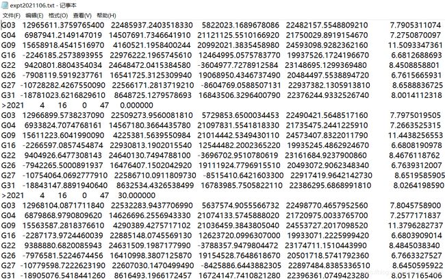
从第二列开始,依次是X坐标、Y坐标、Z坐标、伪距和权值,由于不需要一“>”开头的那一行,所以在处理的时候去掉。将每个历元都分开成一个单独的csv文件,这样方便计算不同历元的坐标,处理这个文件的代码如下所示:
main_file = open("你的所在文件路径\\expt2021106.txt", 'r')
i = 0
for lines in main_file:
    if lines[0] == '>':
        i += 1
        continue
    file = open("C:\\Users\\13499\\Desktop\\Data\\" + str(i) + ".csv", 'a')
    file.write(lines.replace('   ', ',').replace(',,, ', ',').replace(',,,', ',').replace('  ', ',').replace(',,', ','))
    file.close()

main_file.close()
处理完之后,每个历元的数据都被单独分成了一个csv文件,如下图所示:
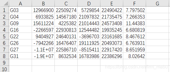
这样就方便遍历计算了。
三、计算代码分析
3.1 坐标系转换模块——coordinate_transport
此部分就是将空间直角坐标系转为经纬度坐标系,即:XYZ→BLH,涉及到大地测量学的知识,此处不多赘述,直接放上代码:
# -*- coding: utf-8 -*-

import math


def xyz2blh(xyz):
    blh = [0, 0, 0]
    a = 6378137.0
    f = 1.0 / 298.257223563
    e2 = f * (2 - f)
    r2 = xyz[0] * xyz[0] + xyz[1] * xyz[1]
    z = xyz[2]
    zk = 0.0

    while abs(z - zk) >= 0.0001:
        zk = z
        sinp = z / math.sqrt(r2 + z * z)
        v = a / math.sqrt(1.0 - e2 * sinp * sinp)
        z = xyz[2] + v * e2 * sinp

    if r2 > 1E-12:
        blh[0] = math.atan(z / math.sqrt(r2))
        blh[1] = math.atan2(xyz[1], xyz[0])
    else:
        if r2 > 0:
            blh[0] = math.pi / 2.0
        else:
            blh[0] = -math.pi / 2.0
        blh[1] = 0.0

    blh[2] = math.sqrt(r2 + z * z) - v
    return blh
3.2 读取数据和伪距单点定位计算模块——Point_positioning
首先,导入numpy库和刚刚在coordinate_transport模块中写好的坐标转换函数xyz2blh。
import numpy as np
from coordinate_transport import xyz2blh
由于涉及到角度转换,所以先写一个将弧度制转为十进制的函数:
def rad2deg(rad):
    """
    this function can turn rad_type angle into deg_type angle
    :param rad: rad_type angle
    :return: deg_type angle
    """
    return rad / np.pi * 180
读入数据的时候,由于读入时为字符串,而计算时需要使用浮点数,所以先写一个将字符串列表转为浮点数列表的函数:
def str2float(li):
    """
    turn string list into float list
    :param li: string list
    :return: float list
    """
    for i in range(len(li)):
        li[i] = float(li[i])
    return li
然后是读取数据的代码,在3.1中,我们已经将每个历元的数据都处理成了单独的csv文件,所以只要单个读取再遍历即可。这里我们将读取一个csv文件的代码封装成函数,返回五个列表,分别为X,Y,Z坐标、伪距和方差。
def read_data(data_path):
    """
    this function can read the data I need for this task
    :param data_path: the path of csv file
    :return: the data in csv file
    """
    file = open(data_path, 'r')
    x = []
    y = []
    z = []
    c_range = []
    var = []
    line_num = 0
    for lines in file:
        temp_str = lines.strip('\n')
        temp_list = temp_str.split(",")
        x.append(temp_list[1])
        y.append(temp_list[2])
        z.append(temp_list[3])
        c_range.append(temp_list[4])
        var.append(temp_list[5])
        line_num += 1
        if line_num == 4:
            break
    file.close()
    x = str2float(x)
    y = str2float(y)
    z = str2float(z)
    c_range = str2float(c_range)
    var = str2float(var)
    return x, y, z, c_range, var
做完准备工作之后,就可以开始写伪距单点定位的计算代码了。伪距单点定位其实就是一个最小而成求解的过程,非常简单。首先定义光速,并且将初始坐标设为(0,0,0)
def point_position(x, y, z, c_range, var):
    c = 299792458
    x0, y0, z0 = 0, 0, 0  # initial coordinate
然后组成设计矩阵A和观测向量L,组成的方法直接照着书上的公式就可以了,这里不细讲:
R = np.mat(np.zeros((4, 1)))  # approximate geometric distance
l = np.mat(np.zeros((4, 1)))  # first column of the design matrix
m = np.mat(np.zeros((4, 1)))  # second column of the design matrix
n = np.mat(np.zeros((4, 1)))  # third column of the design matrix
L = np.mat(np.zeros((4, 1)))  # observation vector
for j in range(len(x)):
    R[j, 0] = np.sqrt((x[j] - x0) ** 2 + (y[j] - y0) ** 2 + (z[j] - z0) ** 2)
    l[j, 0] = (x[j] - x0) / R[j, 0]
    m[j, 0] = (y[j] - y0) / R[j, 0]
    n[j, 0] = (z[j] - z0) / R[j, 0]
    L[j, 0] = c_range[j] - R[j, 0]

A = np.hstack((l, m, n, np.mat([[c], [c], [c], [c]])))  # design matrix
然后组成权阵P,权阵的组成就是将上面读取的权值放在对角线上即可:
P = np.mat(
            [[var[0], 0., 0., 0.], [0., var[1], 0., 0.], [0., 0., var[2], 0.], [0., 0., 0., var[3]]])  # weigh
然后利用最小二乘法计算改正数:
X = -(A.T * P * A).I * (A.T * P * L)
每次循环之后都将初始坐标加上改正数,经过五次循环后大概就收敛了。
x0, y0, z0 = x0 + X[0, 0], y0 + X[1, 0], z0 + X[2, 0]
至此,已经计算出了坐标,单点定位基本实现了。接下来是一些DOP值的计算,利用误差传播定律计算即可
QY = (A.T * P * A).I  # cofactor matrix
    QX = QY[[0, 1, 2]]
    QX = QX[:, [0, 1, 2]]

    blh = xyz2blh([x0, y0, z0])  # B--rad,L--rad
    B, L = blh[0], blh[1]
    rotate = np.mat([[-np.sin(B) * np.cos(L), -np.sin(B) * np.sin(L), np.cos(B)], [-np.sin(L), np.cos(L), 0],
                     [np.cos(B) * np.cos(L), np.sin(B) * np.sin(L), np.sin(B)]])  # rotate matrix
    QR = rotate * QX * rotate.T
    HDOP = np.sqrt(QR[0, 0] + QR[1, 1])
    VDOP = np.sqrt(QR[2, 2])
    PDOP = np.sqrt(QX[0, 0] + QX[1, 1] + QX[2, 2])
    TDOP = np.sqrt(QY[3, 3])
    GDOP = np.sqrt(QX[0, 0] + QX[1, 1] + QX[2, 2] + QY[3, 3])
3.3 结果输出模块——Main
这里我们要将每个历元的计算结果绘制成图,所以先导入绘图库和刚刚写好的单点定位模块
from Point_positioning import read_data, point_position
import matplotlib.pyplot as plt
定义主函数main,一共有1284个历元,所以利用一个遍历,计算处每个历元的X、Y、Z坐标,并分别存如三个列表中,然后修改plt.plot(hengzhou,X)中的X即可绘制出X或Y或Z随不同历元的变化图。
def main():
    X = []
    Y = []
    Z = []
    for i in range(0, 1284):
        path = 'C:\\Users\\13499\\Desktop\\Data\\' + str(i) + '.csv'
        x, y, z, c_range, var = read_data(path)
        x0, y0, z0 = point_position(x, y, z, c_range, var)
        X.append(x0)
        Y.append(y0)
        Z.append(z0)

    hengzhou = [i for i in range(0, 1284)]
    plt.plot(hengzhou, X)
    plt.show()
然后运行主函数即可:
if __name__ == '__main__':
    main()
四、结果展示
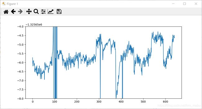
计算出的X坐标随历元变化图如下图所示:
Y坐标:
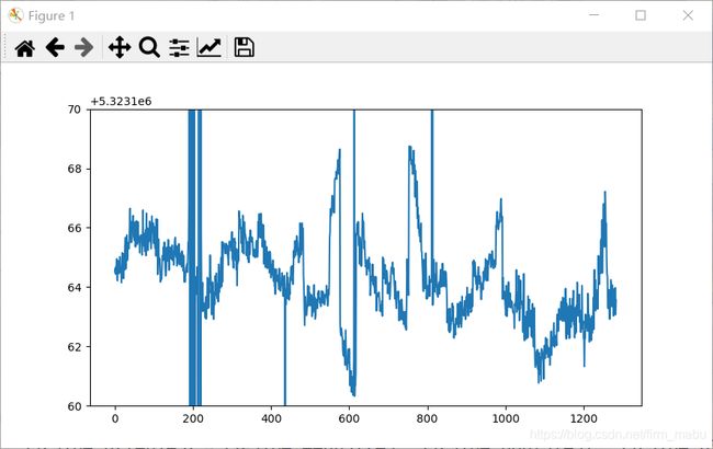
Z坐标:
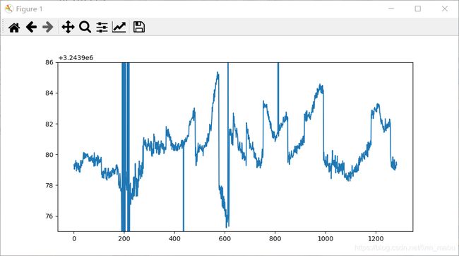
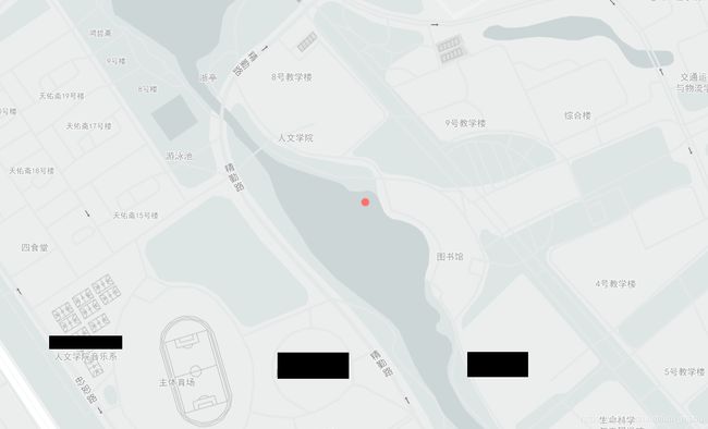
从上面可以看出,有几个历元的数据是有问题的,但是问题出在哪我暂时也找不到,这就是需要继续学习的地方吧。从上面计算出的数据挑出一个显示在地图上,发现在成都某说唱学校的图书馆附近(图中红色的点):
五、感想心得
终于写出来一次大作业了,我也太菜了。
六、源代码
6.1 坐标转换模块
# -*- coding: utf-8 -*-

import math


def xyz2blh(xyz):
    blh = [0, 0, 0]
    a = 6378137.0
    f = 1.0 / 298.257223563
    e2 = f * (2 - f)
    r2 = xyz[0] * xyz[0] + xyz[1] * xyz[1]
    z = xyz[2]
    zk = 0.0

    while abs(z - zk) >= 0.0001:
        zk = z
        sinp = z / math.sqrt(r2 + z * z)
        v = a / math.sqrt(1.0 - e2 * sinp * sinp)
        z = xyz[2] + v * e2 * sinp

    if r2 > 1E-12:
        blh[0] = math.atan(z / math.sqrt(r2))
        blh[1] = math.atan2(xyz[1], xyz[0])
    else:
        if r2 > 0:
            blh[0] = math.pi / 2.0
        else:
            blh[0] = -math.pi / 2.0
        blh[1] = 0.0

    blh[2] = math.sqrt(r2 + z * z) - v
    return blh
6.2 单点定位模块
# -*- coding: utf-8 -*-

import numpy as np
from coordinate_transport import xyz2blh


def rad2deg(rad):
    """
    this function can turn rad_type angle into deg_type angle
    :param rad: rad_type angle
    :return: deg_type angle
    """
    return rad / np.pi * 180


def str2float(li):
    """
    turn string list into float list
    :param li: string list
    :return: float list
    """
    for i in range(len(li)):
        li[i] = float(li[i])
    return li


def read_data(data_path):
    """
    this function can read the data I need for this task
    :param data_path: the path of csv file
    :return: the data in csv file
    """
    file = open(data_path, 'r')
    x = []
    y = []
    z = []
    c_range = []
    var = []
    line_num = 0
    for lines in file:
        temp_str = lines.strip('\n')
        temp_list = temp_str.split(",")
        x.append(temp_list[1])
        y.append(temp_list[2])
        z.append(temp_list[3])
        c_range.append(temp_list[4])
        var.append(temp_list[5])
        line_num += 1
        if line_num == 4:
            break
    file.close()
    x = str2float(x)
    y = str2float(y)
    z = str2float(z)
    c_range = str2float(c_range)
    var = str2float(var)
    return x, y, z, c_range, var


def point_position(x, y, z, c_range, var):
    c = 299792458
    x0, y0, z0 = 0, 0, 0  # initial coordinate
    for i in range(5):
        R = np.mat(np.zeros((4, 1)))  # approximate geometric distance
        l = np.mat(np.zeros((4, 1)))  # first column of the design matrix
        m = np.mat(np.zeros((4, 1)))  # second column of the design matrix
        n = np.mat(np.zeros((4, 1)))  # third column of the design matrix
        L = np.mat(np.zeros((4, 1)))  # observation vector
        for j in range(len(x)):
            R[j, 0] = np.sqrt((x[j] - x0) ** 2 + (y[j] - y0) ** 2 + (z[j] - z0) ** 2)
            l[j, 0] = (x[j] - x0) / R[j, 0]
            m[j, 0] = (y[j] - y0) / R[j, 0]
            n[j, 0] = (z[j] - z0) / R[j, 0]
            L[j, 0] = c_range[j] - R[j, 0]

        A = np.hstack((l, m, n, np.mat([[c], [c], [c], [c]])))  # design matrix
        P = np.mat(
            [[var[0], 0., 0., 0.], [0., var[1], 0., 0.], [0., 0., var[2], 0.], [0., 0., 0., var[3]]])  # weight matrix
        X = -(A.T * P * A).I * (A.T * P * L)
        x0, y0, z0 = x0 + X[0, 0], y0 + X[1, 0], z0 + X[2, 0]
    QY = (A.T * P * A).I  # cofactor matrix
    QX = QY[[0, 1, 2]]
    QX = QX[:, [0, 1, 2]]

    blh = xyz2blh([x0, y0, z0])  # B--rad,L--rad
    B, L = blh[0], blh[1]
    rotate = np.mat([[-np.sin(B) * np.cos(L), -np.sin(B) * np.sin(L), np.cos(B)], [-np.sin(L), np.cos(L), 0],
                     [np.cos(B) * np.cos(L), np.sin(B) * np.sin(L), np.sin(B)]])  # rotate matrix
    QR = rotate * QX * rotate.T
    HDOP = np.sqrt(QR[0, 0] + QR[1, 1])
    VDOP = np.sqrt(QR[2, 2])
    PDOP = np.sqrt(QX[0, 0] + QX[1, 1] + QX[2, 2])
    TDOP = np.sqrt(QY[3, 3])
    GDOP = np.sqrt(QX[0, 0] + QX[1, 1] + QX[2, 2] + QY[3, 3])
    # print(HDOP, VDOP, PDOP, TDOP, GDOP)
    return x0, y0, z0
6.3 计算绘图模块
from Point_positioning import read_data, point_position
import matplotlib.pyplot as plt


def main():
    X = []
    Y = []
    Z = []
    for i in range(0, 1284):
        path = 'C:\\Users\\13499\\Desktop\\Data\\' + str(i) + '.csv'
        x, y, z, c_range, var = read_data(path)
        x0, y0, z0 = point_position(x, y, z, c_range, var)
        X.append(x0)
        Y.append(y0)
        Z.append(z0)

    hengzhou = [i for i in range(0, 1284)]
    plt.plot(hengzhou, Z)
    plt.show()


if __name__ == '__main__':
    main()