08_09_4_Semi-supervised_PCA_reconstru_K-Means_Clustering_Gaussian Mixture_Anomaly Detection_Dirichle

cp11_Working with Unlabeled Data_Clustering Analysis_Kmeans_hierarchical_dendrogram_heat map_DBSCAN
https://blog.csdn.net/Linli522362242/article/details/105813977

08_Dimensionality Reduction_svd_Kernel_pca_make_swiss_roll_subplot2grid_IncrementalPCA_memmap_LLE
https://blog.csdn.net/Linli522362242/article/details/105139547

08_09_Dimension Reduction_Gaussian mixture_kmeans++_extent_tick_params_silhouette_image segment_tSNE
https://blog.csdn.net/Linli522362242/article/details/105722461

08_09_2_Semi-supervised(kmeans+log_reg)_propagate_EM_np.percentile_DBSCAN+knn_Spectral_BayesianGaussianMixture_Likelihood
https://blog.csdn.net/Linli522362242/article/details/105973507

08_Dimensionality Reduction_04_Mixture Models and EM_K-means_Image segmentation_compression
https://blog.csdn.net/Linli522362242/article/details/106036242

Exercises
1. How would you define clustering? Can you name a few clustering algorithms?

     In Machine Learning, clustering is the unsupervised task of grouping similar instances together. The notion of similarity depends on the task at hand: for example, in some cases two nearby instances will be considered similar, while in others similar instances may be far apart as long as they belong to the same densely packed group. Popular clustering algorithms include K-Means, DBSCAN, agglomerative clustering, BIRCH, Mean-Shift, affinity propagation, and spectral clustering.

2. What are some of the main applications of clustering algorithms?

     The main applications of clustering algorithms include data analysis, customer segmentation, recommender systems, search engines, image segmentation, semisupervised learning, dimensionality reduction, anomaly detection, and novelty detection.

3. Describe two techniques to select the right number of clusters when using K-Means.

     The elbow rule is a simple technique to select the number of clusters when using K-Means: just plot the inertia (the mean squared distance from each instance to its nearest centroid) as a function of the number of clusters, and find the point in the curve where the inertia stops dropping fast (the “elbow”). This is generally close to the optimal number of clusters. https://blog.csdn.net/Linli522362242/article/details/105722461
Figure 9-8. When plotting the inertia as a function of the number of clusters k, the curve often contains an inflexion曲折变化 point called the “elbow”
Figure 9-9. Selecting the number of clusters k using the silhouette score

     Another approach is to plot the silhouette score( (b-a)/max(a,b)) as a function of the number of clusters. There will often be a peak, and the optimal number of clusters is generally nearby. The silhouette score is the mean silhouette coefficient over all instances.The silhouette coefficient can vary between -1 and +1: a coefficient close to +1 means that the instance is well inside its own cluster and far from other clusters, while a coefficient close to 0 means that it is close to a cluster boundary, and finally a coefficient close to -1 means that the instance may have been assigned to the wrong cluster(since instances that are very close to another cluster).).

You may also plot the silhouette diagrams and perform a more thorough analysis.
Figure 9-10. Analyzing the silhouette diagrams for various values of k

• The shape’s height indicates the number of instances the cluster contains,
• and its width represents the sorted silhouette coefficients of the instances in the cluster (wider is better).
• The dashed line indicates the mean silhouette coefficient(over all the instances). 

The vertical dashed lines represent the silhouette score for each number of clusters.

     When most of the instances in a cluster have a lower coefficient than this score (i.e., if many of the instances stop short of the dashed line, ending to the left of it), then the cluster is rather bad since this means its instances are much too close to other clusters. We can see that when k = 3 and when k = 6, we get bad clusters.
But when k = 4 or k = 5, the clusters look pretty good: most instances extend beyond the dashed line, to the right and closer to 1.0. When k = 4, the cluster at index 1 (the third from the top) is rather big. When k = 5, all clusters have similar sizes. So, even though the overall silhouette score from k = 4 is slightly greater than for k = 5, it seems like a good idea to use k = 5 to get clusters of similar sizes(height indicates the number of instances the cluster contains)

4. What is label propagation? Why would you implement it, and how?

     Labeling a dataset is costly and time-consuming. Therefore, it is common to have plenty of unlabeled instances, but few labeled instances. Label propagation is a technique that consists in copying some (or all) of the labels from the labeled instances to similar unlabeled instances. This can greatly extend the number of labeled instances, and thereby allow a supervised algorithm to reach better performance (this is a form of semi-supervised learning). One approach is to use a clustering algorithm such as K-Means on all the instances, then for each cluster find the most common label or the label of the most representative instance (i.e., the one closest to the centroid) and propagate it to the unlabeled instances in the same cluster.

 

• Let's find 50 representative images, then label them https://blog.csdn.net/Linli522362242/article/details/105973507
  Let's see how we can do better. First, let's cluster the training set into 50 clusters, then for each cluster let's find the image closest to the centroid (k=50). We will call these images the representative images: # Unsupervised-learning

k=50
 
# cluster the training set into 50 clusters
kmeans = KMeans( n_clusters=k, random_state=42 )
# then replace the images with their distances to the 50 clusters' centroids
X_digits_dist = kmeans.fit_transform( X_train )
# X_train.shape       #(1347, 64) #64=8*8 
# X_digits_dist.shape # (1347, 50)
 
# for each cluster let's find the representative image "closest to the centroid"
# Represents the index of the instance closest to the centroid of each cluster
representative_digit_idx = np.argmin( X_digits_dist, axis=0 )
X_representative_digits = X_train[ representative_digit_idx ] #extraction
 
representative_digit_idx

import matplotlib.pyplot as plt
 
plt.figure( figsize=(8,2) )
 
for index, X_representative_digit in enumerate(X_representative_digits):
    plt.subplot( k//10, 10, index+1) # rows, columns, index(start 1)
    plt.imshow( X_representative_digit.reshape(8,8), cmap="binary", interpolation="bilinear" )
    plt.axis("off")
    
plt.show()

• Let’s look at each image and manually label it basd on X_representative_digits OR 50 representative images :

y_representative_digits = np.array([
    0, 1, 3, 2, 7, 6, 4, 6, 9, 5, 
    1, 2, 9, 5, 2, 7, 8, 1, 8, 6, 
    3, 1, 5, 4, 5, 4, 0, 3, 2, 6, 
    1, 7, 7, 9, 1, 8, 6, 5, 4, 8, 
    5, 3, 3, 6, 7, 9, 7, 8, 4, 9
]) #y_train[representative_digit_idx]

• propagating the labels to all the other instances in the same cluster
  The clusters of y_train_propagated and kmeans_labels (###from after trained kmeans###) have a one-to-one correspondence, because it is feasible to use the label(### y_representative_digits[i] ###) of the data point closest to the centroid of the clusters for propagation

  y_train_propagated = np.empty( len(X_train), dtype=np.int32 ) # empty dataset
  # kmeans = KMeans( n_clusters=k, random_state=42 )
  # X_digits_dist = kmeans.fit_transform( X_train ) #distances with 50 centroids
  #  X_train <-- kmeans.labels_ with cluster index(0~49)
  # X_digits_dist.shape # (1347, 50)
   
  ### Represents the index(0~1346) of the instance closest to the centroid of each cluster(0~49)
  # representative_digit_idx = np.argmin( X_digits_dist, axis=0 ) #an index list # 1x50
  # X_representative_digits = X_train[ representative_digit_idx ] # extraction # (50, 64=8x8)
  # plt.imshow( X_representative_digit.reshape(8,8), cmap="binary", interpolation="bilinear" ) 
  #           ==>y_representative_digits
  # iterates all clusters
  for i in range(k): # 0~49                    #cluster index(or i): y or digit
      y_train_propagated[kmeans.labels_ ==i] = y_representative_digits[i]#fill with representative digits(total amount=50 digits with labels)

  log_reg = LogisticRegression( multi_class="ovr", solver="liblinear", random_state=42 )
  log_reg.fit( X_train, y_train_propagated)

  

  log_reg.score(X_test, y_test)

  

• only propagate the labels to the 20th percentile closest to the centroid:

  # # X_digits_dist.shape # (1347, 50 distances to each cluster)
  percentile_closest = 20
                                  # 0,1,2~1346          # values: 0~49   # kmeans.labels_.shape=(1347,)
  X_cluster_dist = X_digits_dist[ np.arange(len(X_train)), kmeans.labels_ ] # copy
  # X_cluster_dist.shape # (1347,) 
  #fill X_cluster_dist with the distance between the closest centroid with each instance
  for i in range(k): # k clusters
                  # kmeans.labels_.shape=(1347,)
      in_cluster = (kmeans.labels_ ==i) #(False, False, True, ...1347...,False)
      cluster_dist = X_cluster_dist[in_cluster]#extraction #[distance,distance,...]
      cutoff_distance = np.percentile(cluster_dist, percentile_closest) #20%
      above_cutoff = (X_cluster_dist > cutoff_distance)
      X_cluster_dist[in_cluster & above_cutoff] = -1

  partially_propagated = ( X_cluster_dist !=-1 )
  X_train_partially_propagated = X_train[partially_propagated] #extraction
  # y_train_propagated: propagating the labels(clusters index) to all the other instances in the same cluster
  y_train_partially_propagated = y_train_propagated[partially_propagated]

  
  log_reg = LogisticRegression( multi_class="ovr", solver="liblinear", random_state=42 )
  log_reg.fit( X_train_partially_propagated, y_train_partially_propagated )

  

  log_reg.score(X_test, y_test)

  

5. Can you name two clustering algorithms that can scale to large datasets? And two that look for regions of high density?

• K-Means and BIRCH scale well to large datasets.
• DBSCAN and Mean-Shift look for regions of high density.

6. Can you think of a use case where active learning would be useful? How would you implement it?

     Active learning is useful whenever you have plenty of unlabeled instances but labeling is costly. In this case (which is very common), rather than randomly selecting instances to label, it is often preferable to perform active learning, where human experts interact with the learning algorithm, providing labels for specific instances when the algorithm requests them. A common approach is uncertainty sampling (see the description in “Active Learning” on https://blog.csdn.net/Linli522362242/article/details/105973507).

• 1. The model is trained on the labeled instances gathered so far, and this model is used to make predictions on all the unlabeled instances.
• 2. The instances for which the model is most uncertain (i.e., when its estimated probability is lowest) are given to the expert to be labeled.
• 3. You iterate this process until the performance improvement stops being worth the labeling effort.

7. What is the difference between anomaly detection and novelty detection?

     Many people use the terms anomaly detection and novelty detection interchangeably, but they are not exactly the same.

• In anomaly detection, the algorithm is trained on a dataset that may contain outliers, and the goal is typically to identify these outliers (within the training set), as well as outliers among new instances.
• In novelty detection, the algorithm is trained on a dataset that is presumed假定 to be “clean,” and the objective is to detect novelties新颖性 strictly among new instances.
• Some algorithms work best for anomaly detection (e.g., Isolation Forest), while others are better suited for novelty detection (e.g., one-class SVM).

8. What is a Gaussian mixture? What tasks can you use it for?

     A Gaussian mixture model (GMM) is a probabilistic model that assumes that the instances were generated from a mixture of several Gaussian distributions whose parameters are unknown. In other words, the assumption is that the data is grouped into a finite number of clusters, each with an ellipsoidal shape (but the clusters may have different ellipsoidal shapes, sizes, orientations, and densities), and we don’t know which cluster each instance belongs to. This model is useful for density estimation, clustering, and anomaly detection.

9. Can you name two techniques to find the right number of clusters when using a Gaussian mixture model?

     One way to find the right number of clusters when using a Gaussian mixture model is to plot the Bayesian information criterion (BIC) or the Akaike information criterion (AIC) as a function of the number of clusters, then choose the number of clusters that minimizes the BIC or AIC.https://blog.csdn.net/Linli522362242/article/details/105973507

# gm = GaussianMixture(n_components=3, n_init=10, random_state=42)
# gm.fit(X)
gm.bic(X)

 

gm.aic(X)

 

# We set n_init=10 to run the k-means clustering algorithms 10 times independently 
# with different random centroids to choose the final model
gm_per_k = [GaussianMixture(n_components=k, n_init=10, random_state=42).fit(X) 
            for k in range(1,11)]
 
bics = [model.bic(X) for model in gm_per_k]
aics = [model.aic(X) for model in gm_per_k]
 
 
plt.figure(figsize=(10,6))
 
plt.plot(range(1,11), bics, "bo-", label="BIC")
plt.plot(range(1,11), aics, "go--", label="AIC")
plt.xlabel("$k$ clusters", fontsize=14)
plt.ylabel("Information Criterion", fontsize=14)
plt.axis([ 1, 9.5, np.min(aics)-50, np.max(aics)+50 ])
plt.annotate("Minimum", xy=(3, bics[2]),  
             xytext=(0.35, 0.6), textcoords="figure fraction", fontsize=14,
             arrowprops=dict(facecolor="black", shrink=0.1)
            )
plt.legend()
plt.title("AIC_BIC_vs_k_diagram")
plt.show()

     Figure 9-21 shows the BIC for different numbers of clusters k. As you can see, both the BIC and the AIC are lowest when k=3, so it is most likely the best choice. Note that we could also search for the best value for the covariance_type hyperparameter. For example, if it is "spherical" rather than "full", then the model has significantly fewer parameters to learn, but it does not fit the data as well.
 Figure 9-21. AIC and BIC for different numbers of clusters k

numpy.Inf : IEEE 754 floating point representation of (positive) infinity（正）无穷大.

Use inf because Inf, Infinity, PINF and infty are aliases for inf. For more details, see inf.

Let's train Gaussian Mixture models with various values of k and measure their BIC:

min_bic = np.infty
 
for k in range(1,11):
    for ct in ("full", "tied", "spherical", "diag"):
        bic = GaussianMixture(n_components=k, n_init=10, covariance_type=ct, random_state=42).fit(X).bic(X)
        
        if bic

 

best_covariance_type

 

Another technique is to use a Bayesian Gaussian mixture model, which automatically selects the number of clusters.

 For example, let’s set the number of clusters to 10 and see what happens:

from sklearn.mixture import BayesianGaussianMixture
 
bgm = BayesianGaussianMixture(n_components=10, n_init=10, random_state=42)
bgm.fit(X)

     The Dirichlet process prior allows to define an infinite number of components and automatically selects the correct number of components: it activates a component only if it is necessary. (different from Dirichlet distribution prior, and weight_concentration_prior https://blog.csdn.net/Linli522362242/article/details/105973507)

np.round(bgm.weights_, 2)

 algorithm automatically detected that only 3 clusters are needed, and
the resulting clusters are almost identical to the ones in Figure 9-17

plt.figure( figsize=(10,5) )
plot_gaussian_mixture(bgm, X)
plt.show()

 

10. Cluster the Olivetti Faces Dataset

     Exercise: The classic Olivetti faces dataset contains 400(=40*10) grayscale 64 × 64(=4096)–pixel images of faces. Each image is flattened to a 1D vector of size 4,096(4096 Dimensionality). 40 different people(40 classes) were photographed (10 times each), and the usual task is to train a model that can predict which person is represented in each picture.
Load the dataset using the sklearn.datasets.fetch_olivetti_faces() function.

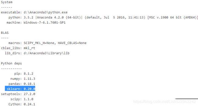
import sklearn #0.20.0

sklearn.show_versions()

from sklearn.datasets import fetch_olivetti_faces

olivetti = fetch_olivetti_faces()

print(olivetti.DESCR)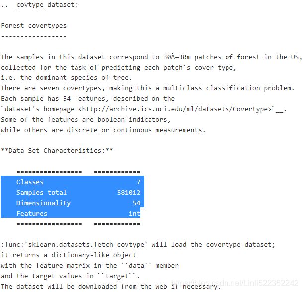

# Reason: http://archive.ics.uci.edu/ml//datasets/Covertype

#But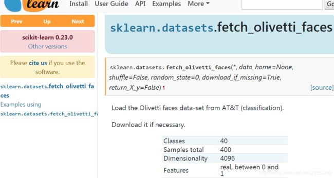
https://mclguide.readthedocs.io/en/latest/sklearn/image.html

Don't worry about the dataset's versions or sklearn's version, Let's see the data.shape

olivetti.data.shape

 

olivetti.target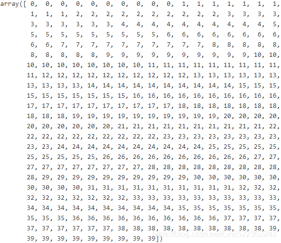

     Exercise: Then - (note that the dataset is already scaled between 0 and 1).

olivetti.data.max(axis=0), olivetti.data.min(axis=0)

     Since the dataset is quite small (400, 4096), you probably want to use stratified sampling to ensure that there are the same number of images per person in each set.

from sklearn.model_selection import StratifiedShuffleSplit

#training_validation_set, test set                
strat_split = StratifiedShuffleSplit( n_splits=1, test_size=40, random_state=42 )
# equal to use a for loop                             #data         #class
# for train_valid_idx, test_idex in strat_split.split(olivetti.data, olivetti.target):
train_valid_idx, test_idex = next( strat_split.split(olivetti.data, olivetti.target) )
X_train_valid = olivetti.data[train_valid_idx]
y_train_valid = olivetti.target[train_valid_idx]
X_test = olivetti.data[test_idex]
y_test = olivetti.target[test_idex]

#training set, validation set
                                                  #the size of validation set
strat_split = StratifiedShuffleSplit( n_splits=1, test_size=80, random_state=43 )
train_idx, valid_idx = next( strat_split.split(X_train_valid, y_train_valid) )
X_train = X_train_valid[train_idx]
y_train = y_train_valid[train_idx]
X_valid = X_train_valid[valid_idx]
y_valid = y_train_valid[valid_idx]

print(X_train.shape, y_train.shape)
print(X_valid.shape, y_valid.shape)
print(X_test.shape, y_test.shape)

To speed things up, we'll reduce the data's dimensionality using PCA:

from sklearn.decomposition import PCA

# PCA assumes that the dataset is centered around the origin. #X_centered = X - X.mean(axis=0)
# The estimated number of components. When n_components is set to 'mle' or a number between 0 and 1 
# (with svd_solver == 'full') this number is estimated from input data.
# preserve 99% of the training set's variance explained  (pca.explained_variance_ratio_>=99%)
# https://blog.csdn.net/Linli522362242/article/details/105139547
pca = PCA(n_components=0.99) #svd_solver='auto'

X_train_pca = pca.fit_transform(X_train)
X_valid_pca = pca.transform(X_valid)
X_test_pca = pca.transform(X_test)

pca.n_components_

 
Exercise: Next, cluster the images using K-Means, and ensure that you have a good number of clusters (using one of the techniques discussed in this chapter).

from sklearn.cluster import KMeans

k_range = range(5,150,5)
kmeans_per_k = []
for k in k_range:
    print("k={}".format(k))
    kmeans = KMeans(n_clusters=k, random_state=42).fit(X_train_pca)
    kmeans_per_k.append(kmeans)

from sklearn.metrics import silhouette_score
# silhouette_score
# This calculates the average silhouette coefficient across all samples, 
# which is equivalent to numpy.mean(silhouette_samples(…)).
silhouette_scores = [silhouette_score(X_train_pca, model.labels_) # metric='euclidean'
                     for model in kmeans_per_k 
                    ]
best_index = np.argmax(silhouette_scores)
best_score = silhouette_scores[best_index]
best_k = k_range[best_index]

plt.figure(figsize=(8,3))
plt.plot(k_range, silhouette_scores, "bo-")
plt.ylabel("Silhouette score", fontsize=14)
plt.xlabel("$k$ clusters", fontsize=14)
plt.plot(best_k, best_score, "rs")
plt.title("silhouette_score_vs_k_diagram")
plt.show()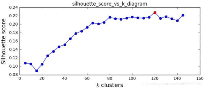

     It looks like the best number of clusters is quite high, at 120. You might have expected it to be 40, since there are 40 different people on the pictures. However, the same person may look quite different on different pictures (e.g., with or without glasses, or simply shifted left or right).

print(best_k)

import matplotlib.pyplot as plt

#inertia_float:Sum of squared distances of samples to their closest cluster center
#return the lowest wc_sse from kmeans
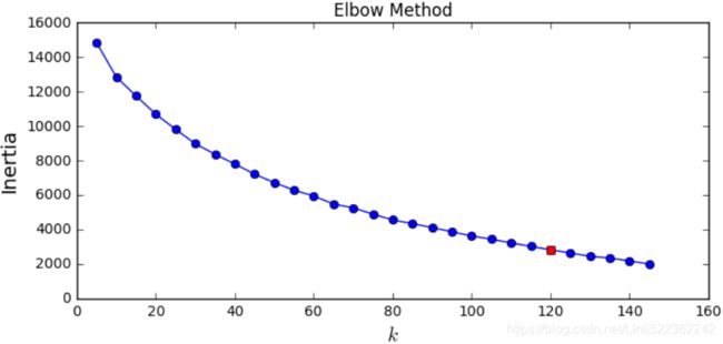
inertias = [ model.inertia_ for model in kmeans_per_k ]

plt.figure(figsize=(8,3.5))
plt.plot(k_range, inertias, "bo-")
plt.plot(best_k, inertias[best_index], "rs")
plt.ylabel("Inertia", fontsize=14)
plt.xlabel("$k$", fontsize=14)
plt.title('Elbow Method')

plt.show()

The optimal number of clusters is not clear on this inertia diagram, as there is no obvious elbow, so let's stick with k=120.

best_model = kmeans_per_k[best_index]

Exercise: Visualize the clusters: do you see similar faces in each cluster?

def plot_faces( faces, labels, n_cols=5 ):
    n_rows = (len(faces)-1) // n_cols+1
    plt.figure( figsize=(n_cols, n_rows*1.1) )
    for index, (face, label) in enumerate( zip(faces, labels) ):
        plt.subplot( n_rows, n_cols, index+1 )
        plt.imshow( face.reshape(64,64), cmap="gray" )
        plt.axis("off")
        plt.title(label)
    plt.show()
    
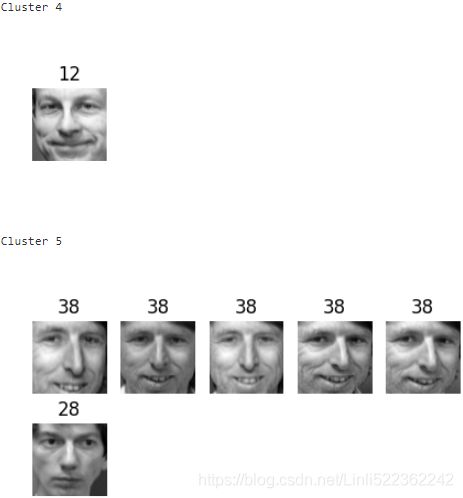
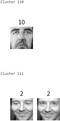
for cluster_id in np.unique( best_model.labels_ ):
    print("Cluster", cluster_id)
    in_cluster = best_model.labels_ == cluster_id
    faces = X_train[in_cluster].reshape(-1,64,64) # extraction
    labels = y_train[in_cluster] # extraction
    plot_faces(faces, labels)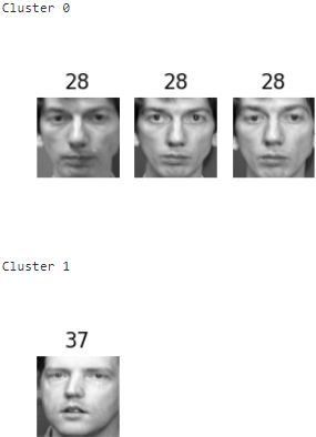

》》... ...
》》 》》 
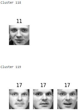
     About 2 out of 3 clusters are useful: that is, they contain at least 2 pictures, and all of the same person. However, the rest of the clusters have either one or more intruders干扰者, or they have just a single picture.

     Clustering images this way may be too imprecise to be directly useful when training a model (as we will see below), but it can be tremendously useful when labeling images in a new dataset: it will usually make labelling much faster.

11. Using Clustering as Preprocessing for Classification

Exercise: Continuing with the Olivetti faces dataset, train a classifier to predict which person is represented in each picture, and evaluate it on the validation set.

from sklearn.ensemble import RandomForestClassifier

clf = RandomForestClassifier( n_estimators=150, random_state=42 )
clf.fit( X_train_pca, y_train )
clf.score( X_valid_pca, y_valid )

Exercise: Next, use K-Means as a dimensionality reduction tool, and train a classifier on the reduced set.

X_train_pca.shape

#Previously, we used kmeans++ to find 120 clusters(best amount of clusters)
X_train_reduced = best_model.transform( X_train_pca ) #use K-Means as a dimensionality reduction tool
X_valid_reduced = best_model.transform( X_valid_pca ) #X_valid_pca.shape(-1,199) --> (-1,120)
X_test_reduced = best_model.transform( X_test_pca )

X_train_reduced.shape

clf = RandomForestClassifier( n_estimators=150, random_state=42 )
clf.fit( X_train_reduced, y_train )

clf.score(X_valid_reduced, y_valid) ## Returns the mean accuracy on the given test data and labels.

    #Note:  clf.score( X_valid_pca, y_valid ) ==0.9  

Yikes! That's not better at all! 

clf.score(X_train_reduced, y_train)

  # overfitting!
Let's see if tuning the number of clusters helps.

     Exercise: Search for the number of clusters that allows the classifier to get the best performance: what performance can you reach?
     We could use a GridSearchCV like we did earlier in this notebook, but since we already have a validation set, we don't need K-fold cross-validation, and we're only exploring a single hyperparameter, so it's simpler to just run a loop manually:

from sklearn.pipeline import Pipeline

for n_clusters in k_range:
    pipeline = Pipeline([ #Via KMeans++ to find the best number of clusters and reduce the dimensions(transform)
            ( "kmeans", KMeans(n_clusters=n_clusters, random_state=n_clusters) ),
            ( "forest_clf", RandomForestClassifier(n_estimators=150, random_state=42) )
        ])
    pipeline.fit(X_train_pca, y_train)
    print( n_clusters, pipeline.score(X_valid_pca, y_valid) ) ##############

     Oh well, even by tuning the number of clusters, we never get beyond 80% accuracy.
### KMeans++ Algorithm through the distances to the nearest cluster's centroid to cluster the samples or datapoints###
Looks like the distances to the cluster centroids are not as informative as the original images.

 

     Exercise: What if you append the features from the reduced set to the original features (again, searching for the best number of clusters)?

X_train_extended = np.c_[X_train_pca, X_train_reduced] #.shape: [ (280, 199),(280, 120) ]
X_valid_extended = np.c_[X_valid_pca, X_valid_reduced]
X_test_extended = np.c_[X_test_pca, X_test_reduced]
X_train_extended.shape

clf = RandomForestClassifier(n_estimators=150, random_state=42)
clf.fit(X_train_extended, y_train)
clf.score(X_valid_extended, y_valid)

     That's a bit better, but still worse than without the cluster features ( clf.score( X_valid_pca, y_valid ) == 0.9 and clf.score(X_valid_reduced, y_valid) == 0.7 ). The clusters are not useful to directly train a classifier in this case (but they can still help when labelling new training instances).

12. A Gaussian Mixture Model for the Olivetti Faces Dataset

     Exercise: Train a Gaussian mixture model on the Olivetti faces dataset. To speed up the algorithm, you should probably reduce the dataset's dimensionality (e.g., use PCA, preserving 99% of the variance).

from sklearn.mixture import GaussianMixture
                    # since 40 persons
gm = GaussianMixture(n_components=40, random_state=42)
y_pred = gm.fit_predict(X_train_pca) # X_train_pca.shape: (280,199)

 

Exercise: Use the model to generate some new faces (using the sample() method),

n_generate_faces = 20
generate_faces_reduced, y_generate_faces = gm.sample( n_samples=n_generate_faces )
generate_faces_reduced.shape, y_generate_faces.shape

 

               and visualize them (if you used PCA, you will need to use its inverse_transform() method). 

generate_faces = pca.inverse_transform( generate_faces_reduced ) 
generate_faces.shape

 # ==64*64

def plot_faces( faces, labels, n_cols=5 ):
    n_rows = (len(faces)-1) // n_cols+1
    plt.figure( figsize=(n_cols, n_rows*1.1) )
    for index, (face, label) in enumerate( zip(faces, labels) ):
        plt.subplot( n_rows, n_cols, index+1 )
        plt.imshow( face.reshape(64,64), cmap="gray" )
        plt.axis("off")
        plt.title(label)
    plt.show()
    
plot_faces(generate_faces, y_generate_faces)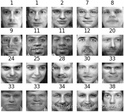

Exercise: Try to modify some images (e.g., rotate, flip, darken) and see if the model can detect the anomalies (i.e., compare the output of the score_samples() method for normal images and for anomalies).
#########################################

                                #(z,x,y)
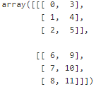
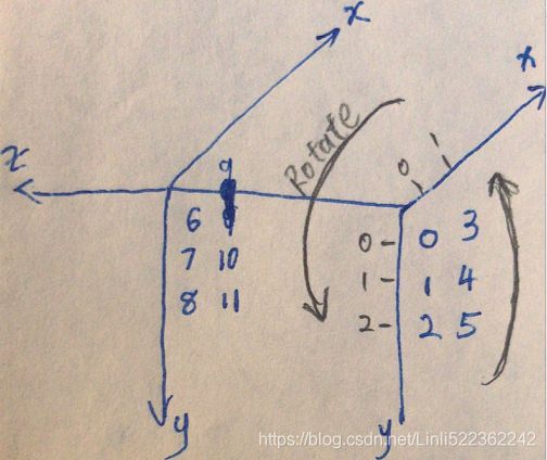
dataset = np.arange(12).reshape( (2,2,3) )
dataset

 

                                    #(z,y,x)
dataset = np.transpose(dataset, axes=[0,2,1])
dataset

Besides, flip

#########################################

Exercise: Try to modify some images (e.g., rotate, flip, darken) (from original dataset) and see if the model can detect the anomalies (i.e., compare the output of the score_samples() method for normal images and for anomalies).

n_rotated = 4         #X_train.shape:(280,4096)                     #z x y  
rotated = np.transpose(X_train[:n_rotated].reshape(-1, 64,64), axes=[0,2,1])
rotated = rotated.reshape(-1,64*64) # rotated face 
y_rotated = y_train[:n_rotated]

n_flipped = 3                        #(3,64,64)
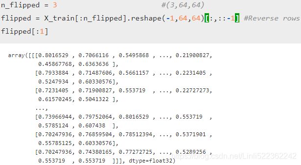
flipped = X_train[:n_flipped].reshape(-1,64,64)[:,::-1] #Reverse rows
flipped = flipped.reshape(-1,64*64) # flipped face
y_flipped = y_train[:n_flipped]

n_darkened =3
darkened = X_train[:n_darkened].copy()
darkened[:,1:-1] *=0.3  #dark
darkened = darkened.reshape(-1,64*64) # darkened face
y_darkened = y_train[:n_darkened]

X_bad_faces = np.r_[rotated, flipped, darkened] # np.r_ for list and return an array
y_bad = np.r_[y_rotated, y_flipped, y_darkened] # np.concatenate([y_rotated, y_flipped, y_darkened]) 

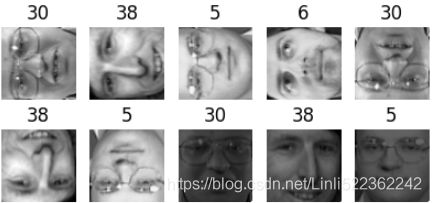
plot_faces(X_bad_faces, y_bad)

Note, the rotation we usually talk about, we must add a flip operation in the code implementation process

X_bad_faces_pca = pca.transform(X_bad_faces)

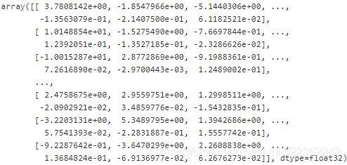
gm.score_samples(X_bad_faces_pca) # Compute the weighted log probabilities for each sample.

https://blog.csdn.net/Linli522362242/article/details/105973507

Compute the weighted log probabilities for a sample:   *==>
* ==> ln ( ) for one sample/instance in a Gaussian mixture mode. (here, we treat  as a weight)
Out:

The bad faces are all considered highly unlikely极不可能发生 by the Gaussian Mixture model.
Compare this to the scores of some training instances:

gm.score_samples(X_train_pca[:10])

13. Using Dimensionality Reduction Techniques for Anomaly Detection

     Exercise: Some dimensionality reduction techniques can also be used for anomaly detection.
     For example, take the Olivetti faces dataset and reduce it with PCA, preserving 99% of the variance. Then compute the reconstruction error for each image. Next, take some of the modified images you built in the previous exercise, and look at their reconstruction error: notice how much larger the reconstruction error is. If you plot a reconstructed image, you will see why: it tries to reconstruct a normal face.

We already reduced the dataset using PCA earlier:

X_train_pca

def reconstruction_errors(pca, X):
    X_pca = pca.transform(X)  #reduce X's dimensions with PCA
    X_reconstructed = pca.inverse_transform(X_pca)
    mse = np.square( X_reconstructed-X ).mean(axis= 1) #==.mean(axis= -1)
    return mse

Then compute the reconstruction error for each image. 

reconstruction_errors(pca, X_train).mean() #hidden default axis=0 since just 1D_array

plot_faces(X_train[:4], y_train) # we just use first 4 faces

plot_faces(  pca.inverse_transform(pca.transform( X_train[:4] )), y_train[:4] )

distortion:  

 
Next, take some of the modified images you built in the previous exercise, and look at their reconstruction error: notice how much larger the reconstruction error is.

reconstruction_errors(pca, X_bad_faces).mean(axis=0)

plot_faces(X_bad_faces, y_bad)

If you plot a reconstructed image, you will see why: it tries to reconstruct a normal face.

#X_bad_faces_pca = pca.transform(X_bad_faces)
X_bad_faces_reconstructed = pca.inverse_transform(X_bad_faces_pca)
plot_faces(X_bad_faces_reconstructed, y_bad)

pca.inverse_transform(X_bad_faces_pca)  tries to reconstruct a normal face, even though we modified images before reducing the dataset' s dimensions with pca.