【书籍阅读 Ch3】Reinforcement Learning An Introduction, 2nd Edition

前言：第1、2章点此进入
注：每一个目录对应的是在pdf的页数（如果LPage就是书左上角的页码 - 因为我发现后面我要在两页之间加空白页 做练习lol 例如：LPage28 就是左上角书页28页，RPage29就是右上角书页29页）；【】这个框架之间有时候是我留的疑问，与一些关于方向上连接的想法 主要集中于无人驾驶的控制层，带问号结束的就是…我的疑问

更新时间：2021/01/19

推荐观看：
1.英文 - PDF链接
2 中文 - 官方京东书籍购买链接
代码参考：
1.github 关于整本书的图python代码
2.github 关于整本书的练习solution参考

回顾与进入

从上一章 我们应该还能记得那个赌博机的例子 bandit 而聪明的你一定发现了 $$A_t\dot{=}\underset{a}{\mathrm{argmax}}{Q}_t(a)$$ 这里我们估计了每个动作a的价值q，然后在这章中，我们需要考虑这个动作在这个状态下的价值，也就是加入了状态这一参数从 $q_{\ast }(a)$ 到 -> 到 $q_{\ast }(s,a)$ 或者是给定最优动作下每个状态的价值 $v_{\ast }(s)$
而MDP是强化学习问题在数学上的理想化形式(mathematically idealized) -【所以相对于其他学习的方式？RL其实是在前面给出了一种数学的解释方式，可解释性更强？】
$$\sum _{s^{\prime }\in S}\sum _{r\in R}p\left(s^{\prime },r|s,a\right)=1\text{for all}s\in S,a\in A(a)$$在马尔可夫决策过程中 这个式子中$p$给出的概率完全刻画了环境的动态特性。所以这个时刻的状态和动作取决于上一个时刻的，This is best viewed a restriction not on the decision process, but on the state 这个限制针对的就是状态，而不是决策的过程。
A state must include information about all aspects of the past agent-environment interaction that make a difference for the future那么这样的状态就是具有马尔可夫性的 Markov property

之后就是对于MDP来说，什么sensory memory control都可以无需公式化，只要介定好了三个东西：action, state, rewards

3.2 Goal and Rewards

首先是第一段自己的想法：At each time step, the reward is a simple number $R_t\in \mathbb{R}$ 【那我们是否可以从这里将reward定义由人为驾驶数据得出的数据分值化成为state】

这本节的最后一段指出：the reward signal is not the place to impart to the agent prior knowledge about how to achieve what we want it to do. 也就是说 我们不应该去引导agent去实现我们想要的目标，而是让它自己探索那个目标【但是这样的话 如果目标不具有独立性，也就是说你的每一步都部分决定了你离目标的距离 这样的情况 难道不应该为这些步骤也赋予一定的reward而使其与远离目标的点做区分吗？】

理由：If achieving these sorts of subgoals were rewarded, then the agent might find a way to achieve them without achieving the real goal.

结论：The reward signal is your way of communicating to the robot what you want it to achieve, not how you want it achieved.【在第17章也进一步的进行了讨论】

3.4 (Lpage 57)

最后的 Thus, we can define the return, in general, according to (3.8), using the convention of omitting episode numbers when they are not needed, and including the possibility that $\gamma =1$ if the sum remains defined【这里的sum remains是指的什么？】
$$G_t\dot{=}\sum _{k=t+1}^T{\gamma }^{k-t-1}{R}_k\text{(3.11)}$$

3.5 Policies and Value Functions

LPage 58: 最后一句 We call estimation methods of this kind Monte Carlo methods because ***
这里的公式3.13与3.11的不同之处在哪里？->一个是episode 有限时间内，3.13是无穷大
$$q_{\pi }(s,a)\doteq {\mathbb{E}}_{\pi }\left[G_t\mid S_t=s,A_t=a\right]={\mathbb{E}}_{\pi }\left[\sum _{k=0}^{\infty }{\gamma }^k{R}_{t+k+1}\mid S_t=s,A_t=a\right]\text{(3.13)}$$
Example 3.5: Grid World 代码：

import matplotlib
import matplotlib.pyplot as plt
import numpy as np
from matplotlib.table import Table

WORLD_SIZE = 5
A_POS = [0, 1]
A_PRIME_POS = [4, 1]
B_POS = [0, 3]
B_PRIME_POS = [2, 3]
DISCOUNT = 0.9

# left, up, right, down
ACTIONS = [np.array([0, -1]),
           np.array([-1, 0]),
           np.array([0, 1]),
           np.array([1, 0])]
ACTIONS_FIGS=[ '←', '↑', '→', '↓']


ACTION_PROB = 0.25


def step(state, action):
    if state == A_POS:
        return A_PRIME_POS, 10
    if state == B_POS:
        return B_PRIME_POS, 5

    next_state = (np.array(state) + action).tolist()
    x, y = next_state
    if x < 0 or x >= WORLD_SIZE or y < 0 or y >= WORLD_SIZE:
        reward = -1.0
        next_state = state
    else:
        reward = 0
    return next_state, reward
    
def figure_3_2():
    value = np.zeros((WORLD_SIZE, WORLD_SIZE))
    while True:
        # keep iteration until convergence
        new_value = np.zeros_like(value)
        for i in range(WORLD_SIZE):
            for j in range(WORLD_SIZE):
                for action in ACTIONS:
                    (next_i, next_j), reward = step([i, j], action)
                    # bellman equation
                    new_value[i, j] += ACTION_PROB * (reward + DISCOUNT * value[next_i, next_j])
        if np.sum(np.abs(value - new_value)) < 1e-4:
            draw_image(np.round(new_value, decimals=2))
            plt.savefig('../images/figure_3_2.png')
            plt.close()
            break
        value = new_value
        
def figure_3_2_linear_system():
    '''
    Here we solve the linear system of equations to find the exact solution.
    We do this by filling the coefficients for each of the states with their respective right side constant.
    '''
    A = -1 * np.eye(WORLD_SIZE * WORLD_SIZE)
    b = np.zeros(WORLD_SIZE * WORLD_SIZE)
    for i in range(WORLD_SIZE):
        for j in range(WORLD_SIZE):
            s = [i, j]  # current state
            index_s = np.ravel_multi_index(s, (WORLD_SIZE, WORLD_SIZE))
            for a in ACTIONS:
                s_, r = step(s, a)
                index_s_ = np.ravel_multi_index(s_, (WORLD_SIZE, WORLD_SIZE))

                A[index_s, index_s_] += ACTION_PROB * DISCOUNT
                b[index_s] -= ACTION_PROB * r

    x = np.linalg.solve(A, b)
    draw_image(np.round(x.reshape(WORLD_SIZE, WORLD_SIZE), decimals=1))
    plt.show()
    
if __name__ == '__main__':
	figure_3_2()
    figure_3_2_linear_system()
    

可以看到动作先在动作库里进行选择，然后再由step改变由这个动作产生的状态，ACTION_PROB是因为书中说明了选择每个action的概率平均0.25，每循环完一次地图的尺寸，更新new_value的值到value然后继续 直到两个差值小于1e-4其实就是value保持不变了就没必要循环了，生成的图如下：

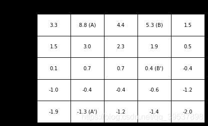
3.6 Optimal Policies and Optimal Value Functions

对于RPage:63 我们可以知道 $v_{\ast }(s)$是最优策略下的value of state，$q_{\ast }(s,a)$是expected return for best action in state s，期望回报(注意reward是一个动作后的收益，return是一系列动作后的回报)
也就是下面的这两个式子
$$\begin{array}{rl}{v}_{\ast }(s)& =\underset{a\in \mathcal{A}(s)}{\max }{q}_{{\pi }_{\ast }}(s,a)\\ & =\underset{a}{\max }{\mathbb{E}}_{{\pi }_{\ast }}\left[G_t\mid S_t=s,A_t=a\right]\\ & =\underset{a}{\max }{\mathbb{E}}_{{\pi }_{\ast }}\left[R_{t+1}+\gamma G_{t+1}\mid S_t=s,A_t=a\right]\\ & =\underset{a}{\max }\mathbb{E}\left[R_{t+1}+\gamma v_{\ast }\left(S_{t+1}\right)\mid S_t=s,A_t=a\right]\\ & =\underset{a}{\max }\sum _{s^{\prime },r}p\left(s^{\prime },r\mid s,a\right)\left[r+\gamma v_{\ast }\left(s^{\prime }\right)\right]\end{array}$$$$\begin{array}{rl}{q}_{\ast }(s,a)& =\mathbb{E}\left[R_{t+1}+\gamma \underset{a^{\prime }}{\max }{q}_{\ast }\left(S_{t+1},a^{\prime }\right)\mid S_t=s,A_t=a\right]\\ & =\sum _{s^{\prime },r}p\left(s^{\prime },r\mid s,a\right)\left[r+\gamma \underset{a^{\prime }}{\max }\left(s^{\prime },a^{\prime }\right)\right]\end{array}$$感觉这幅图很好的描述了 两个式子的关系

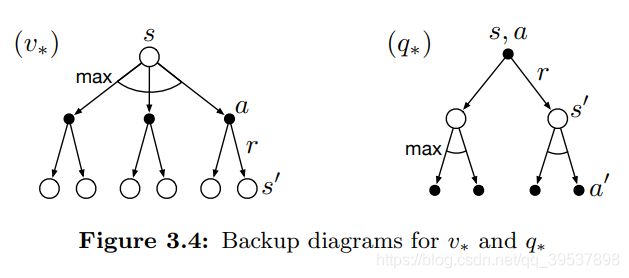
而在这里如果确定好了$v_{\ast }$也就是状态的价值，那policy也就很好确定了 一个状态下有很多个可行action 每一个都对应一个Policy，选择了这个policy也就是选择了这个动作，通过Bellman optimal equation可得。例如 使用单步搜索 也就是每一步我都选择前方价值最大的状态 及状态下的最优动作。而这一节的数学意义就是将未来的价值使用Bellman方程考虑在了value function里。
所以定$v_{\ast }$的意义：我们可以将最优的长期（全局）回报期望值转化为每个状态对应的一个当前局部量计算，也就是单步搜索就可以产生长期最优的动作序列。

Example 3.8: Solving the GridWorld

代码：

import matplotlib
import matplotlib.pyplot as plt
import numpy as np
from matplotlib.table import Table

WORLD_SIZE = 5
A_POS = [0, 1]
A_PRIME_POS = [4, 1]
B_POS = [0, 3]
B_PRIME_POS = [2, 3]
DISCOUNT = 0.9

# left, up, right, down
ACTIONS = [np.array([0, -1]),
           np.array([-1, 0]),
           np.array([0, 1]),
           np.array([1, 0])]
ACTIONS_FIGS=[ '←', '↑', '→', '↓']


ACTION_PROB = 0.25


def step(state, action):
    if state == A_POS:
        return A_PRIME_POS, 10
    if state == B_POS:
        return B_PRIME_POS, 5

    next_state = (np.array(state) + action).tolist()
    x, y = next_state
    if x < 0 or x >= WORLD_SIZE or y < 0 or y >= WORLD_SIZE:
        reward = -1.0
        next_state = state
    else:
        reward = 0
    return next_state, reward


def draw_image(image):
    fig, ax = plt.subplots()
    ax.set_axis_off()
    tb = Table(ax, bbox=[0, 0, 1, 1])

    nrows, ncols = image.shape
    width, height = 1.0 / ncols, 1.0 / nrows

    # Add cells
    for (i, j), val in np.ndenumerate(image):

        # add state labels
        if [i, j] == A_POS:
            val = str(val) + " (A)"
        if [i, j] == A_PRIME_POS:
            val = str(val) + " (A')"
        if [i, j] == B_POS:
            val = str(val) + " (B)"
        if [i, j] == B_PRIME_POS:
            val = str(val) + " (B')"
        
        tb.add_cell(i, j, width, height, text=val,
                    loc='center', facecolor='white')
        

    # Row and column labels...
    for i in range(len(image)):
        tb.add_cell(i, -1, width, height, text=i+1, loc='right',
                    edgecolor='none', facecolor='none')
        tb.add_cell(-1, i, width, height/2, text=i+1, loc='center',
                    edgecolor='none', facecolor='none')

    ax.add_table(tb)

def draw_policy(optimal_values):
    fig, ax = plt.subplots()
    ax.set_axis_off()
    tb = Table(ax, bbox=[0, 0, 1, 1])

    nrows, ncols = optimal_values.shape
    width, height = 1.0 / ncols, 1.0 / nrows

    # Add cells
    for (i, j), val in np.ndenumerate(optimal_values):
        next_vals=[]
        for action in ACTIONS:
            next_state, _ = step([i, j], action)
            next_vals.append(optimal_values[next_state[0],next_state[1]])

        best_actions=np.where(next_vals == np.max(next_vals))[0]
        val=''
        for ba in best_actions:
            val+=ACTIONS_FIGS[ba]
        
        # add state labels
        if [i, j] == A_POS:
            val = str(val) + " (A)"
        if [i, j] == A_PRIME_POS:
            val = str(val) + " (A')"
        if [i, j] == B_POS:
            val = str(val) + " (B)"
        if [i, j] == B_PRIME_POS:
            val = str(val) + " (B')"
        
        tb.add_cell(i, j, width, height, text=val,
                loc='center', facecolor='white')

    # Row and column labels...
    for i in range(len(optimal_values)):
        tb.add_cell(i, -1, width, height, text=i+1, loc='right',
                    edgecolor='none', facecolor='none')
        tb.add_cell(-1, i, width, height/2, text=i+1, loc='center',
                   edgecolor='none', facecolor='none')

    ax.add_table(tb)

def figure_3_5():
    value = np.zeros((WORLD_SIZE, WORLD_SIZE))
    while True:
        # keep iteration until convergence
        new_value = np.zeros_like(value)
        for i in range(WORLD_SIZE):
            for j in range(WORLD_SIZE):
                values = []
                for action in ACTIONS:
                    (next_i, next_j), reward = step([i, j], action)
                    # value iteration
                    values.append(reward + DISCOUNT * value[next_i, next_j])#这里就是对应的公式3.17
                new_value[i, j] = np.max(values)#对应公式3.18 也就是选最大value的最大
        if np.sum(np.abs(new_value - value)) < 1e-4:
            draw_image(np.round(new_value, decimals=2))
            draw_policy(new_value)
            break
        value = new_value
if __name__ == '__main__':
	figure_3_5()

因为这里的action选择不再根据概率去选择（或者说因为在例3.5中说了 四个动作的概率均相同），也就是我们计算一个状态内的所有动作的value

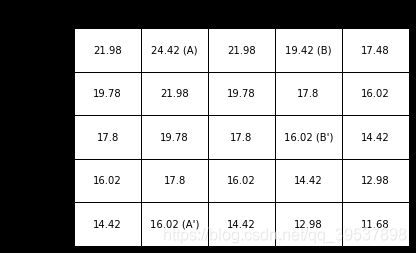
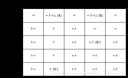
LPage: 66

如果需要使用$v_{\ast }(s)$ 显式求解Bellman equation是需要预估所有的可能性，计算每种可能性出现的概率及expected reward，需要同时满足这三个条件：

• 准确知道环境的动态变化特性 (dynamics of the environment)
• 足够的算力（enough computational resources to complete the computation of the solution）
• 马尔科夫性质（Markov property）
  但是这三个条件通常来说很难同时满足例如围棋

据有人计算：围棋棋盘横竖各有19条线，共有361个落子点，双方交替落子，这意味着围棋总共可能有$10^{171}$(1后面有171个零)种可能性。这个数字到底有多大，你可能没有感觉。我们可以告诉你，宇宙中的原子总数是$10^{80}$(1后面80个零)，即使穷尽整个宇宙的物质也不能存下围棋的所有可能性。

如果这么多的状态用贝尔曼方程求解$v_{\ast }$或者是求解$q_{\ast }$都是不行的，所以通常使用近似或机器/深度学习去解决。

3.8 Summary

Elements

• actions are the choices made by the agent
• states are the basis for making the choices
• rewards are the basis for evaluating the choices
• policy is a stochastic rule by which the agent selects actions as a function of states.
• return is the function of future rewards that the agent seeks to maximize.
• Everything inside the agent is completely known and controllable by the agent
• Everything outside is incompletely controllable but may or may not be completely known.

Value Function

• A policy’s value functions assign to each state, or state–action pair, the expected return from that state, or state–action pair, given that the agent uses the policy.
• The optimal value functions assign to each state, or state–action pair, the largest expected return achievable by any policy.

All Exercise Part

Exercise 3.1: Devise three example tasks of your own that fit into the MDP framework, identifying for each its states, actions, and rewards. Make the three examples as different from each other as possible. The framework is abstract and flexible and can be applied in many different ways. Stretch its limits in some way in at least one of your examples.
The MDP framework is describe by the formula as below:
$$p(s^{\prime },r|s,a)\dot{=}\text{Pr}\{S_t=s^{\prime },R_t=r|S_{t-1}=s,A_{t-s}=a\}$$

• an agent to escape the maze of grid.
  State: position in the maze and the time in the maze
  Action: move action (north, west, south, east)
  Reward: reach the goal +1; otherwise 0; timeout -1
• an agent try to learn which arm to use to grasp a glass.
  State: arm position
  Action: adjust arm position
  Reward: grasp a glass success +1; otherwise 0; glass fall down -1
• an agent to decide how to hot its heater that could make water 60 degrees hot.
  State: water temperature and heater degree
  Action: change the header degree
  Reward: 60 degrees +1; otherwise 0; <40 or >80 -1
  【迷宫的那一个例子在后面3.7中提及会有问题 如果不加timeout -1】

Exercise 3.2: Is the MDP framework adequate to usefully represent all goal-directed learning tasks? Can you think of any clear exceptions?

• don’t have enough calculation power to find all $s$ and $r$ 也就是状态情况太多了，例如围棋的虽然是RL框架但是使用的DL做的framework而不是MDP，原因就是因为算力更不上
• 对于那些具有goal-directed tasks但是他的state不具有Markov property 例如射击类的游戏 你无法观测到all information of the environments.
  

Exercise 3.3: Consider the problem of driving. You could define the actions in terms of the accelerator, steering wheel, and brake, that is, where your body meets the machine. Or you could define them farther out—say, where the rubber meets the road, considering your actions to be tire torques. Or you could define them farther in—say, where your brain meets your body, the actions being muscle twitches to control your limbs. Or you could go to a really high level and say that your actions are your choices of where to drive. What is the right level, the right place to draw the line between agent and environment? On what basis is one location of the line to be preferred over another? Is there any fundamental reason for preferring one location over another, or is it a free choice?
This problem is asking the proper line to define the environment and the agent. To my understanding, the line should be divided such that the effect of agent’s action $a$ on state $s$ could be observed in some way.
也就是说我们选定的action的影响需要在状态里进行提现并且还能观测到observed
对于fundamental reason我写的是(\大笑)：Think about how human will do the job about the action

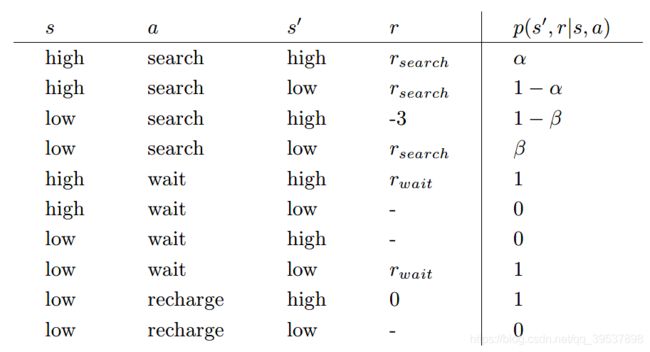
Exercise 3.4: Give a table analogous to that in Example 3.3, but for $p(s^{\prime },r|s,a)$. It should have columns for $s,a,s^{\prime },r$ and $p(s^{\prime },r|s,a)$, and a row for every 4-tuple for which $p(s^{\prime },r|s,a)>0$.
也就是由Example 3.3的表格演化而来的 把 $r$提前

Exercise 3.5: The equations in Section 3.1 are for the continuing case and need to be modified (very slightly) to apply to episodic tasks. Show that you know the modifications needed by giving the modified version of (3.3).
原来的公式：$$\sum _{s^{\prime }\in S}\sum _{r\in R}p\left(s^{\prime },r|s,a\right)=1\text{for all}s\in S,a\in A(a)$$为了适用于episodic tasks：$$\sum _{s^{\prime }\in S^{+}}\sum _{r\in R}p\left(s^{\prime },r|s,a\right)=1\text{for all}s\in S,a\in A(a)$$不同之处在于$S$到$S^{+}$；$S$代表的是non-terminal states，$S^{+}$代表的是All states include terminal state

Exercise 3.6: Suppose you treated pole-balancing as an episodic task but also used discounting, with all rewards zero except for $-1$ upon failure. What then would the return be at each time? How does this return differ from that in the discounted, continuing formulation of this task?
First review the episodic task without discount:$$G_t\dot{=}{R}_{t+1}+R_{t+2}+\cdots +R_T$$Add discount into this formula will be:
$$G_t\dot{=}{R}_{t+1}+\gamma R_{t+2}+\cdots +{\gamma }^{T-(t+1)}{R}_T=\sum _{k=0}^{T-(t+1)}{\gamma }^k{R}_{k+t+1}$$因为这是0 for success; -1 for failure，所以如果在第K时刻失败了，收益和应该是：$-{\gamma }^K$，在K时刻前都是$0$；这是对于episodic，对于continuing task:$$G_t\dot{=}{R}_{t+1}+\gamma R_{t+2}+\cdots =\sum _{k=0}^{\infty }{\gamma }^k{R}_{k+t+1}$$但是如果也是在K时刻的时候失败了，收益和也是$-{\gamma }^K$，而在K时刻前都是$0$，所以没有不同

Exercise 3.7: Imagine that you are designing a robot to run a maze. You decide to give it a reward of $+1$ for escaping from the maze and a reward of zero at all other times. The task seems to break down naturally into episodes—the successive runs through the maze—so you decide to treat it as an episodic task, where the goal is to maximize expected total reward (3.7). After running the learning agent for a while, you find that it is showing no improvement in escaping from the maze. What is going wrong? Have you effectively communicated to the agent what you want it to achieve?
应该要限定时间，同样的要加入discount，越接近出口的步数的reward越大

引用答案：If you do not use to implement the discount, the maximum return is always 1 regardless the time the agent spends. The correct way to communicate the agent is to add -1 punishment to each time step before the escape or adding the discount.

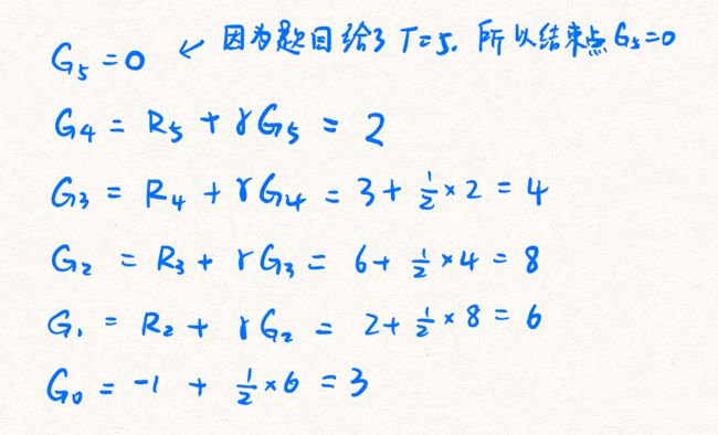
Exercise 3.8: Suppose γ = 0.5 and the following sequence of rewards is received $R_1=-1,R_2=2,R_3=6,R_4=3$, and $R_5=2$, with $T=5$. What are $G_0,G_1,...,G_5$? Hint: Work backwards.

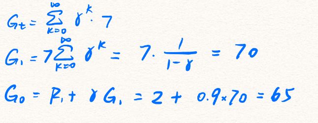
Exercise 3.9: Suppose γ = 0.9 and the reward sequence is R1 = 2 followed by an infinite sequence of 7s. What are G1 and G0?

Exercise 3.10: Prove the second equality in (3.10)

Exercise 3.11: If the current state is $S_t$, and actions are selected according to stochastic policy $\pi$, then what is the expectation of $R_{t+1}$ in terms of $\pi$ and the four-argument function $p$ (3.2)?
$$\mathbb{E}(R_t|S_t=s)=\sum _a\pi (a|S_t)\sum _{s^{\prime },r}p\left(s^{\prime },r|s,a\right)r$$

Exercise 3.12: Give an equation for $v_{\pi }$ in terms of $q_{\pi }$ and $\pi$
$$v_{\pi }(s)\dot{=}\sum _a\pi (a|s)q_{\pi }(s,a)$$

Exercise 3.13: Give an equation for $q_{\pi }$ in terms of $v_{\pi }$ and the four-argument $p$.
$$q_{\pi }(s,a)=\sum _{s^{\prime },r}p\left(s^{\prime },r\mid s,a\right)\left[r+\gamma v_{\pi }\left(s^{\prime }\right)\right]$$

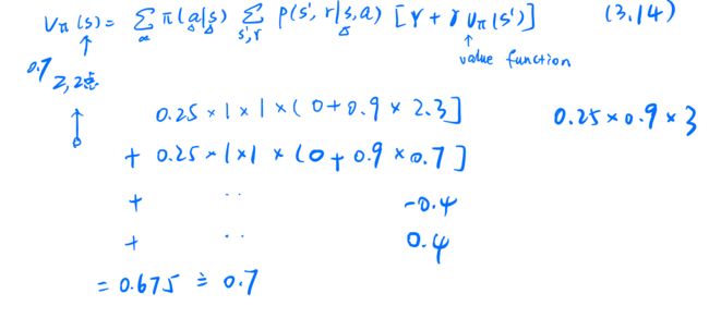
Exercise 3.14: The Bellman equation (3.14) must hold for each state for the value function $v_{\pi }$ shown in Figure 3.2 (right) of Example 3.5. Show numerically that this equation holds for the center state, valued at +0.7, with respect to its four neighboring states, valued at +2.3, +0.4, 0.4, and +0.7. (These numbers are accurate only to one decimal place.)

Exercise 3.15: In the gridworld example, rewards are positive for goals, negative for running into the edge of the world, and zero the rest of the time. Are the signs of these rewards important, or only the intervals between them? Prove, using (3.8), that adding a constant c to all the rewards adds a constant, $v_c$, to the values of all states, and thus does not affect the relative values of any states under any policies. What is $v_c$ in terms of $c$ and $\gamma$?

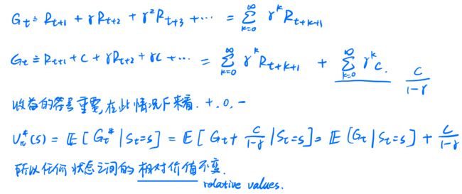
Exercise 3.16: Now consider adding a constant $c$ to all the rewards in an episodic task, such as maze running. Would this have any effect, or would it leave the task unchanged as in the continuing task above? Why or why not? Give an example.
看这个常数是否会让现有的negative reward变为positive 因为如果变到了正数reward 对于gridworld这种episodic 用正负来加速完成任务的操作 是会有影响的，此外 负的ward如果保持负，整体的学习也会受到变慢的影响 因为value的值下降的不够快（对于正负来说）

引用答案It is a similar question as one before. The sign of reward is critical in episodic task because episodic task uses negative reward to accelerate the agent finishing the task. Thus, adding a constant C, if changing the sign, would have an impact on how agent moves. Furthermore, if the negative reward remains negative but the value of it shrinks too much, it will give a wrong signal to the agent that the time of completing the job is not that important.

Exercise 3.17: What is the Bellman equation for action values, that is, for $q_{\pi }$? It must give the action value $q_{\pi }(s,a)$ in terms of the action values, $q_{\pi }(s^{\prime },a^{\prime })$, of possible successors to the state–action pair $(s,a)$. Hint: the backup diagram to the right corresponds to this equation. Show the sequence of equations analogous to (3.14), but for action values.
$$\begin{array}{rl}{q}_{\pi }(s,a)& =\mathbb{E}[G_t|S_t=s,A_t=a]\\ & =\mathbb{E}\left[R_{t+1}+\gamma G_{t+1}\left(S_{t+1}\right)\mid S_t=s,A_t=a\right]\\ & =\sum _{s^{\prime },r}p\left(s^{\prime },r\mid s,a\right)\left[r+\gamma \sum _{a^{\prime }}\pi (a^{\prime }|s^{\prime })q_{\pi }(s^{\prime },a^{\prime })\right]\end{array}$$

Exercise 3.18: The value of a state depends on the values of the actions possible in that state and on how likely each action is to be taken under the current policy. We can think of this in terms of a small backup diagram rooted at the state and considering each possible action: