机器学习之降维压缩数据
特征提取:将原始数据压缩为低纬度的
5.1用主成分分析实现无监督降维
5.1完成以下步骤:
- 标准化数据
- 构建协方差矩阵
- 获取协方差矩阵特征值和特征向量
- 以降序对特征值排序,从而对特征排序
import pandas as pd
import numpy as np
import matplotlib.pyplot as plt
df=pd.read_csv('wine-Copy1.data',names=['分类标签','酒精','苹果酸',
                                  '灰','灰的碱度','镁','总酚','黄酮类化合物',
                                  '非黄烷类酚类','原花青素','色彩强度',
                                  '色调','稀释酒','脯氨酸'])
df.head()
| 分类标签 | 酒精 | 苹果酸 | 灰 | 灰的碱度 | 镁 | 总酚 | 黄酮类化合物 | 非黄烷类酚类 | 原花青素 | 色彩强度 | 色调 | 稀释酒 | 脯氨酸 | |
|---|---|---|---|---|---|---|---|---|---|---|---|---|---|---|
| 0 | 1 | 14.23 | 1.71 | 2.43 | 15.6 | 127 | 2.80 | 3.06 | 0.28 | 2.29 | 5.64 | 1.04 | 3.92 | 1065 |
| 1 | 1 | 13.20 | 1.78 | 2.14 | 11.2 | 100 | 2.65 | 2.76 | 0.26 | 1.28 | 4.38 | 1.05 | 3.40 | 1050 |
| 2 | 1 | 13.16 | 2.36 | 2.67 | 18.6 | 101 | 2.80 | 3.24 | 0.30 | 2.81 | 5.68 | 1.03 | 3.17 | 1185 |
| 3 | 1 | 14.37 | 1.95 | 2.50 | 16.8 | 113 | 3.85 | 3.49 | 0.24 | 2.18 | 7.80 | 0.86 | 3.45 | 1480 |
| 4 | 1 | 13.24 | 2.59 | 2.87 | 21.0 | 118 | 2.80 | 2.69 | 0.39 | 1.82 | 4.32 | 1.04 | 2.93 | 735 |
from sklearn.model_selection import train_test_split
X=df.iloc[:,1:].values
y=df.iloc[:,0].values
X_train,X_test,y_train,y_test=train_test_split(X,y,test_size=0.3,stratify=y,
                                              random_state=0)
print(X_train.shape)
print(X_test.shape)
print(y_train.shape)
print(y_test.shape)
(124, 13)
(54, 13)
(124,)
(54,)
#标准化
from sklearn.preprocessing import StandardScaler
sc=StandardScaler()
X_train_std=sc.fit_transform(X_train)
X_test_std=sc.transform(X_test)
def cov(m, y=None, rowvar=True, bias=False, ddof=None, fweights=None,aweights=None)
m:一维或则二维的数组,默认情况下每一行代表一个变量(属性),每一列代表一个观测
#获取协方差矩阵的特征值和特征向量
cov_mat=np.cov(X_train_std.T)
cov_mat.shape
(13, 13)
w,v = numpy.linalg.eig(a) 计算方形矩阵a的特征值和右特征向量
参数:
a : 待求特征值和特征向量的方阵。
返回:
w: 多个特征值组成的一个矢量。备注:多个特征值并没有按特定的次序排列。特征值中可能包含复数。

v: 多个特征向量组成的一个矩阵。每一个特征向量都被归一化了。第i列的特征向量v[:,i]对应第i个特征值w[i]。
————————————————
eigen_vals,eigen_vecs=np.linalg.eig(cov_mat)
eigen_vals
array([4.84274532, 2.41602459, 1.54845825, 0.96120438, 0.84166161,
       0.6620634 , 0.51828472, 0.34650377, 0.3131368 , 0.10754642,
       0.21357215, 0.15362835, 0.1808613 ])
eigen_vecs.shape
(13, 13)
总方差和解释方差
tot=sum(eigen_vals)
var_exp=[(i/tot) for i in sorted(eigen_vals,reverse=True)]
var_exp
[0.36951468599607645,
 0.18434927059884165,
 0.11815159094596986,
 0.07334251763785471,
 0.06422107821731672,
 0.05051724484907654,
 0.03954653891241449,
 0.026439183169220035,
 0.02389319259185293,
 0.016296137737251016,
 0.013800211221948418,
 0.01172226244308596,
 0.008206085679091375]
#累计解释方差
cum_var_exp=np.cumsum(var_exp)
cum_var_exp
array([0.36951469, 0.55386396, 0.67201555, 0.74535807, 0.80957914,
       0.86009639, 0.89964293, 0.92608211, 0.9499753 , 0.96627144,
       0.98007165, 0.99179391, 1.        ])
#coding:utf-8
import matplotlib.pyplot as plt
plt.rcParams['font.sans-serif']=['SimHei'] #用来正常显示中文标签
plt.rcParams['axes.unicode_minus']=False #用来正常显示负号
#有中文出现的情况,需要u'内容


plt.bar(range(1,14),var_exp,alpha=0.5,align='center',
       label='解释方差')
plt.step(range(1,14),cum_var_exp,label='累计解释方差',color='k')
plt.xlabel('主成分索引')
plt.xlabel('解释方差比率')
plt.legend(loc='best')

[
特征变换
- 选择与前k个特征值对应的特征向量,其中k为新特征子空间的维数(k≤d)
- 用前k个特征向量构造投影矩阵W
- 用投影矩阵W变换d维输入数据集X以获得新的k维特征子空间
#做一个(特征值,特征向量)元组
eigen_pairs=[(np.abs(eigen_vals[i]),eigen_vecs[:,i]) for i in range(len(eigen_vals))]
eigen_pairs[0]
(4.842745315655895,
 array([-0.13724218,  0.24724326, -0.02545159,  0.20694508, -0.15436582,
        -0.39376952, -0.41735106,  0.30572896, -0.30668347,  0.07554066,
        -0.32613263, -0.36861022, -0.29669651]))
#对特征值排序
eigen_pairs.sort(key=lambda k:k[0],reverse=True)
#选用前两个最大特征值的特征向量
w=np.hstack((eigen_pairs[0][1][:,np.newaxis],
           eigen_pairs[1][1][:,np.newaxis]))
w#得到13×2的投影矩阵
array([[-0.13724218,  0.50303478],
       [ 0.24724326,  0.16487119],
       [-0.02545159,  0.24456476],
       [ 0.20694508, -0.11352904],
       [-0.15436582,  0.28974518],
       [-0.39376952,  0.05080104],
       [-0.41735106, -0.02287338],
       [ 0.30572896,  0.09048885],
       [-0.30668347,  0.00835233],
       [ 0.07554066,  0.54977581],
       [-0.32613263, -0.20716433],
       [-0.36861022, -0.24902536],
       [-0.29669651,  0.38022942]])
这里只选择了两个,实际中,主成分的数量必需通过在计算效率和分类器性能平衡来确定
两个新特征的的样本向量
$ X^{'}=XW $
#获得2维度的数据集
X_train_pca=X_train_std.dot(w)
X_train_pca.shape
(124, 2)
#可视化实现
colors=['r','b','g']
markers=['s','x','o']
for l,c,m in zip(np.unique(y_train),colors,markers):
    plt.scatter(X_train_pca[y_train==l,0],X_train_pca[y_train==l,1],
               c=c,label=l,marker=m)

plt.xlabel('PC 1')
plt.ylabel('PC 2')
plt.legend(loc='best')
plt.show()

PCA是不使用任何分类标签的无监督学习技术
sklearn实现
#边界决策的可视化

from matplotlib.colors import ListedColormap

def plot_decision_regions(X,y,classifier,test_idx=None,resolution=0.02):

##简历颜色产生器和颜色绘图板
    markers=('s','x','o','^','y')
    colors=('red','blue','lightgreen','gray','cyan')
    cmap=ListedColormap(colors[:len(np.unique(y))])

##画出决策边界

    x1_min,x1_max=X[:,0].min()-1,X[:,0].max()+2
    x2_min,x2_max=X[:,1].min()-1,X[:,1].max()+2
    xx1,xx2=np.meshgrid(np.arange(x1_min,x1_max,resolution),
                       np.arange(x2_min,x2_max,resolution))
    z=classifier.predict(np.array([xx1.ravel(),xx2.ravel()]).T)
    z=z.reshape(xx1.shape)
    plt.contourf(xx1,xx2,z,alpha=0.2,cmap=cmap)
    plt.xlim(xx1.min(),xx2.max())
    plt.ylim(xx2.min(),xx2.max())

    #绘出样例
    for idx,c1 in enumerate(np.unique(y)):
        plt.scatter(x=X[y==c1,0],y=X[y==c1,1],
                   alpha=0.8,c=cmap(idx),
                   marker=markers[idx],label=c1)

    #绘出测试样例
    if test_idx:
        X_test,y_test=X[test_idx,:],y[test_idx]
        plt.scatter(X_test[:,0],X_test[:,1],c='',
                   alpha=0.1,linewidth=1,marker='o',label='test set',
                    edgecolors='black',s=150)
from sklearn.linear_model import LogisticRegression
from sklearn.decomposition import PCA
from sklearn.metrics import accuracy_score

#PCA降维
pca=PCA(n_components=2)

X_train_pca=pca.fit_transform(X_train_std)
X_test_pca=pca.transform(X_test_std)

#训练LogisticRegression模型
lr=LogisticRegression(C=1.1)
lr.fit(X_train_pca,y_train)

#测试集和训练集准确率
pred1=lr.predict(X_train_pca)
accuracy1=accuracy_score(y_train,pred1)
print('训练集准确率:'+"{}".format(accuracy1))

pred2=lr.predict(X_test_pca)
accuracy2=accuracy_score(y_test,pred2)
print('测试集准确率:'+"{}".format(accuracy2))
训练集准确率:0.9838709677419355
测试集准确率:0.9259259259259259
#训练集决策区域
plot_decision_regions(X_train_pca,y_train,classifier=lr)
plt.xlabel('PC 1')
plt.ylabel('PC 2')
plt.legend(loc='best')
plt.show()
*c* argument looks like a single numeric RGB or RGBA sequence, which should be avoided as value-mapping will have precedence in case its length matches with *x* & *y*.  Please use the *color* keyword-argument or provide a 2-D array with a single row if you intend to specify the same RGB or RGBA value for all points.
*c* argument looks like a single numeric RGB or RGBA sequence, which should be avoided as value-mapping will have precedence in case its length matches with *x* & *y*.  Please use the *color* keyword-argument or provide a 2-D array with a single row if you intend to specify the same RGB or RGBA value for all points.
*c* argument looks like a single numeric RGB or RGBA sequence, which should be avoided as value-mapping will have precedence in case its length matches with *x* & *y*.  Please use the *color* keyword-argument or provide a 2-D array with a single row if you intend to specify the same RGB or RGBA value for all points.
#测试集决策区域
plot_decision_regions(X_test_pca,y_test,classifier=lr)
plt.xlabel('PC 1')
plt.ylabel('PC 2')
plt.legend(loc='best')
plt.show()
*c* argument looks like a single numeric RGB or RGBA sequence, which should be avoided as value-mapping will have precedence in case its length matches with *x* & *y*.  Please use the *color* keyword-argument or provide a 2-D array with a single row if you intend to specify the same RGB or RGBA value for all points.
*c* argument looks like a single numeric RGB or RGBA sequence, which should be avoided as value-mapping will have precedence in case its length matches with *x* & *y*.  Please use the *color* keyword-argument or provide a 2-D array with a single row if you intend to specify the same RGB or RGBA value for all points.
*c* argument looks like a single numeric RGB or RGBA sequence, which should be avoided as value-mapping will have precedence in case its length matches with *x* & *y*.  Please use the *color* keyword-argument or provide a 2-D array with a single row if you intend to specify the same RGB or RGBA value for all points.
5.2基于线性判别分析的有监督数据压缩
线性判别方法:提高计算效率和减少维数过高引起的过拟合
LDA是有监督的方法
##手动实现LDA

#标准化前面已经实现

#计算散步矩阵
np.set_printoptions(precision=4)
mean_vecs=[]
for label in range(1,4):
    mean_vecs.append(np.mean(X_train_std[y_train==label],axis=0))
    print("{}{}{}".format('MV',label,mean_vecs[label-1]))
MV1[ 0.9066 -0.3497  0.3201 -0.7189  0.5056  0.8807  0.9589 -0.5516  0.5416
  0.2338  0.5897  0.6563  1.2075]
MV2[-0.8749 -0.2848 -0.3735  0.3157 -0.3848 -0.0433  0.0635 -0.0946  0.0703
 -0.8286  0.3144  0.3608 -0.7253]
MV3[ 0.1992  0.866   0.1682  0.4148 -0.0451 -1.0286 -1.2876  0.8287 -0.7795
  0.9649 -1.209  -1.3622 -0.4013]
mean_vecs
[array([ 0.9066, -0.3497,  0.3201, -0.7189,  0.5056,  0.8807,  0.9589,
        -0.5516,  0.5416,  0.2338,  0.5897,  0.6563,  1.2075]),
 array([-0.8749, -0.2848, -0.3735,  0.3157, -0.3848, -0.0433,  0.0635,
        -0.0946,  0.0703, -0.8286,  0.3144,  0.3608, -0.7253]),
 array([ 0.1992,  0.866 ,  0.1682,  0.4148, -0.0451, -1.0286, -1.2876,
         0.8287, -0.7795,  0.9649, -1.209 , -1.3622, -0.4013])]
S_W=np.zeros((13,13))
d=13
for label,mv in zip(range(1,4),mean_vecs):
    class_scatter=np.zeros((d,d))
    for row in X_train_std[y_train==label]:
        row,mv=row.reshape(d,1),mv.reshape(d,1)
        class_scatter=class_scatter+(row-mv).dot((row-mv).T)
    S_W=S_W+class_scatter
print("{}{}{}{}".format('within-class matrix:',S_W.shape[0],'X',S_W.shape[1]))
within-class matrix:13X13
y_train
array([3, 1, 1, 1, 3, 2, 2, 3, 2, 2, 2, 1, 2, 3, 1, 3, 2, 1, 3, 3, 2, 1,
       2, 2, 2, 2, 3, 1, 2, 2, 1, 1, 3, 1, 2, 1, 1, 2, 3, 3, 1, 3, 3, 3,
       1, 2, 3, 3, 2, 3, 2, 2, 2, 1, 2, 2, 3, 3, 2, 1, 1, 2, 3, 3, 2, 1,
       2, 2, 2, 1, 1, 1, 1, 1, 3, 1, 2, 3, 2, 2, 3, 1, 2, 1, 2, 2, 3, 2,
       1, 1, 1, 3, 2, 1, 1, 2, 2, 3, 3, 2, 1, 1, 2, 2, 3, 1, 3, 1, 2, 2,
       2, 2, 1, 3, 1, 1, 1, 1, 2, 2, 3, 3, 2, 2], dtype=int64)
print("{}{}".format('Class label distribution',np.bincount(y_train)[1:]))
Class label distribution[41 50 33]
#由于样本分布不均,除以各类的n,每个类别散步矩阵相当于协方差矩阵
S_W=np.zeros((13,13))
for label,mv in zip(range(1,4),mean_vecs):
    class_scatter=np.cov(X_train_std[y_train==label].T)
    S_W+=class_scatter
print('{}{}{}{}'.format('Scaled within-class scater matrix:',
                       S_W.shape[0],'X',S_W.shape[1]))
Scaled within-class scater matrix:13X13
#类间散步矩阵
mean_overall=np.mean(X_train_std,axis=0)
d=13
S_B=np.zeros((13,13))
for i,mean_vec in enumerate(mean_vecs):
    n=X_train[y_train==i+1,:].shape[0]
    mean_vec=mean_vec.reshape(d,1)
    mean_overall=mean_overall.reshape(d,1)
    S_B=S_B+n*(mean_vec-mean_overall).dot((mean_vec-mean_overall).T)
print('{}{}{}{}'.format('between-class scatter matrix:',
                         S_B.shape[0],'X',S_B.shape[1]))
between-class scatter matrix:13X13
在新的特征子空间选择线性判别式
计 算 S w − 1 S B 特 征 值 和 特 征 向 量 计算S_{w}^{-1}S_{B}特征值和特征向量 计算Sw−1SB特征值和特征向量
#计算特征值和特征向量
eigen_vals,eigen_vecs=np.linalg.eig(np.linalg.inv(S_W).dot(S_B))
eigen_vals#出现了复数
array([ 0.0000e+00+0.0000e+00j,  1.7276e+02+0.0000e+00j,
        3.4962e+02+0.0000e+00j, -3.7853e-14+0.0000e+00j,
       -2.1174e-14+0.0000e+00j, -2.9948e-15+1.4866e-14j,
       -2.9948e-15-1.4866e-14j,  1.2667e-14+4.8950e-15j,
        1.2667e-14-4.8950e-15j,  7.5878e-15+0.0000e+00j,
       -2.9162e-15+5.1358e-15j, -2.9162e-15-5.1358e-15j,
       -2.2564e-15+0.0000e+00j])
eigen_vecs
array([[ 0.7517+0.j    , -0.4092+0.j    , -0.1481+0.j    ,
         0.406 +0.j    , -0.5115+0.j    , -0.6795+0.j    ,
        -0.6795-0.j    ,  0.6167+0.j    ,  0.6167-0.j    ,
         0.7528+0.j    ,  0.6923+0.j    ,  0.6923-0.j    ,
         0.7594+0.j    ],
       [-0.0834+0.j    , -0.1577+0.j    ,  0.0908+0.j    ,
         0.153 +0.j    , -0.1468+0.j    ,  0.1224+0.0641j,
         0.1224-0.0641j, -0.0988+0.0079j, -0.0988-0.0079j,
        -0.0926+0.j    , -0.1152+0.051j , -0.1152-0.051j ,
        -0.0752+0.j    ],
       [-0.2406+0.j    , -0.3537+0.j    , -0.0168+0.j    ,
         0.2157+0.j    ,  0.0056+0.j    ,  0.0873+0.0821j,
         0.0873-0.0821j, -0.2082-0.047j , -0.2082+0.047j ,
        -0.2838+0.j    , -0.3075-0.1804j, -0.3075+0.1804j,
        -0.2155+0.j    ],
       [ 0.2515+0.j    ,  0.3223+0.j    ,  0.1484+0.j    ,
         0.1153+0.j    , -0.1081+0.j    , -0.3026-0.0141j,
        -0.3026+0.0141j,  0.0359+0.1655j,  0.0359-0.1655j,
         0.2738+0.j    ,  0.2521-0.0098j,  0.2521+0.0098j,
         0.2746+0.j    ],
       [-0.0586+0.j    , -0.0817+0.j    , -0.0163+0.j    ,
         0.0043+0.j    , -0.1021+0.j    ,  0.0499+0.0023j,
         0.0499-0.0023j, -0.0757-0.0479j, -0.0757+0.0479j,
        -0.0627+0.j    ,  0.0819-0.0293j,  0.0819+0.0293j,
        -0.0827+0.j    ],
       [ 0.1027+0.j    ,  0.0842+0.j    ,  0.1913+0.j    ,
        -0.038 +0.j    ,  0.2103+0.j    , -0.1432+0.0557j,
        -0.1432-0.0557j,  0.1065-0.1211j,  0.1065+0.1211j,
         0.0217+0.j    ,  0.1051+0.033j ,  0.1051-0.033j ,
         0.0831+0.j    ],
       [ 0.0109+0.j    ,  0.2823+0.j    , -0.7338+0.j    ,
        -0.5208+0.j    , -0.1468+0.j    , -0.0806-0.0204j,
        -0.0806+0.0204j, -0.0264+0.2665j, -0.0264-0.2665j,
         0.0449+0.j    , -0.0057+0.0149j, -0.0057-0.0149j,
         0.0139+0.j    ],
       [-0.025 +0.j    , -0.0102+0.j    , -0.075 +0.j    ,
        -0.0864+0.j    , -0.0279+0.j    ,  0.0336-0.0378j,
         0.0336+0.0378j, -0.1637-0.058j , -0.1637+0.058j ,
        -0.0851+0.j    , -0.0068-0.0514j, -0.0068+0.0514j,
        -0.0205+0.j    ],
       [ 0.0611+0.j    ,  0.0907+0.j    ,  0.0018+0.j    ,
         0.1421+0.j    , -0.0711+0.j    , -0.0529+0.0346j,
        -0.0529-0.0346j,  0.087 +0.0359j,  0.087 -0.0359j,
         0.0471+0.j    ,  0.0416+0.0129j,  0.0416-0.0129j,
         0.1022+0.j    ],
       [-0.0726+0.j    , -0.2152+0.j    ,  0.294 +0.j    ,
        -0.0811+0.j    , -0.2123+0.j    , -0.0033-0.1045j,
        -0.0033+0.1045j, -0.0395+0.0271j, -0.0395-0.0271j,
        -0.0533+0.j    , -0.0443+0.0641j, -0.0443-0.0641j,
        -0.0811+0.j    ],
       [ 0.1757+0.j    ,  0.2747+0.j    , -0.0328+0.j    ,
        -0.0103+0.j    , -0.3724+0.j    , -0.1923-0.061j ,
        -0.1923+0.061j ,  0.1121-0.2787j,  0.1121+0.2787j,
         0.1673+0.j    ,  0.1886+0.0468j,  0.1886-0.0468j,
         0.1603+0.j    ],
       [-0.0943+0.j    , -0.0124+0.j    , -0.3547+0.j    ,
         0.6254+0.j    , -0.1993+0.j    ,  0.137 -0.0395j,
         0.137 +0.0395j, -0.1668+0.0864j, -0.1668-0.0864j,
        -0.0855+0.j    , -0.0947-0.0672j, -0.0947+0.0672j,
        -0.0816+0.j    ],
       [-0.4933+0.j    , -0.5958+0.j    , -0.3915+0.j    ,
        -0.2319+0.j    ,  0.6322+0.j    ,  0.5491+0.0017j,
         0.5491-0.0017j, -0.5103+0.0514j, -0.5103-0.0514j,
        -0.4639+0.j    , -0.4818+0.005j , -0.4818-0.005j ,
        -0.4818+0.j    ]])
note
Above, I used the numpy.linalg.eig function to decompose the symmetric covariance matrix into its eigenvalues and eigenvectors.
>>> eigen_vals, eigen_vecs = np.linalg.eig(cov_mat)
This is not really a “mistake,” but probably suboptimal. It would be better to use
numpy.linalg.eigh in such cases, which has been designed for Hermetian matrices. The latter always returns real eigenvalues; whereas the numerically less stable np.linalg.eig can decompose nonsymmetric square matrices, you may find that it returns complex eigenvalues in certain cases. (S.R.)
#对特征值排序
eigen_pairs=[(np.abs(eigen_vals[i]),eigen_vecs[:,i]) for i in range(len(eigen_vals))]
eigen_pairs
[(0.0,
  array([ 0.7517+0.j, -0.0834+0.j, -0.2406+0.j,  0.2515+0.j, -0.0586+0.j,
          0.1027+0.j,  0.0109+0.j, -0.025 +0.j,  0.0611+0.j, -0.0726+0.j,
          0.1757+0.j, -0.0943+0.j, -0.4933+0.j])),
 (172.76152218979388,
  array([-0.4092+0.j, -0.1577+0.j, -0.3537+0.j,  0.3223+0.j, -0.0817+0.j,
          0.0842+0.j,  0.2823+0.j, -0.0102+0.j,  0.0907+0.j, -0.2152+0.j,
          0.2747+0.j, -0.0124+0.j, -0.5958+0.j])),
 (349.6178089059939,
  array([-0.1481+0.j,  0.0908+0.j, -0.0168+0.j,  0.1484+0.j, -0.0163+0.j,
          0.1913+0.j, -0.7338+0.j, -0.075 +0.j,  0.0018+0.j,  0.294 +0.j,
         -0.0328+0.j, -0.3547+0.j, -0.3915+0.j])),
 (3.7853134512521556e-14,
  array([ 0.406 +0.j,  0.153 +0.j,  0.2157+0.j,  0.1153+0.j,  0.0043+0.j,
         -0.038 +0.j, -0.5208+0.j, -0.0864+0.j,  0.1421+0.j, -0.0811+0.j,
         -0.0103+0.j,  0.6254+0.j, -0.2319+0.j])),
 (2.117398448224407e-14,
  array([-0.5115+0.j, -0.1468+0.j,  0.0056+0.j, -0.1081+0.j, -0.1021+0.j,
          0.2103+0.j, -0.1468+0.j, -0.0279+0.j, -0.0711+0.j, -0.2123+0.j,
         -0.3724+0.j, -0.1993+0.j,  0.6322+0.j])),
 (1.5164618894178885e-14,
  array([-0.6795+0.j    ,  0.1224+0.0641j,  0.0873+0.0821j, -0.3026-0.0141j,
          0.0499+0.0023j, -0.1432+0.0557j, -0.0806-0.0204j,  0.0336-0.0378j,
         -0.0529+0.0346j, -0.0033-0.1045j, -0.1923-0.061j ,  0.137 -0.0395j,
          0.5491+0.0017j])),
 (1.5164618894178885e-14,
  array([-0.6795-0.j    ,  0.1224-0.0641j,  0.0873-0.0821j, -0.3026+0.0141j,
          0.0499-0.0023j, -0.1432-0.0557j, -0.0806+0.0204j,  0.0336+0.0378j,
         -0.0529-0.0346j, -0.0033+0.1045j, -0.1923+0.061j ,  0.137 +0.0395j,
          0.5491-0.0017j])),
 (1.3579567140455979e-14,
  array([ 0.6167+0.j    , -0.0988+0.0079j, -0.2082-0.047j ,  0.0359+0.1655j,
         -0.0757-0.0479j,  0.1065-0.1211j, -0.0264+0.2665j, -0.1637-0.058j ,
          0.087 +0.0359j, -0.0395+0.0271j,  0.1121-0.2787j, -0.1668+0.0864j,
         -0.5103+0.0514j])),
 (1.3579567140455979e-14,
  array([ 0.6167-0.j    , -0.0988-0.0079j, -0.2082+0.047j ,  0.0359-0.1655j,
         -0.0757+0.0479j,  0.1065+0.1211j, -0.0264-0.2665j, -0.1637+0.058j ,
          0.087 -0.0359j, -0.0395-0.0271j,  0.1121+0.2787j, -0.1668-0.0864j,
         -0.5103-0.0514j])),
 (7.587760371654683e-15,
  array([ 0.7528+0.j, -0.0926+0.j, -0.2838+0.j,  0.2738+0.j, -0.0627+0.j,
          0.0217+0.j,  0.0449+0.j, -0.0851+0.j,  0.0471+0.j, -0.0533+0.j,
          0.1673+0.j, -0.0855+0.j, -0.4639+0.j])),
 (5.906039984472233e-15,
  array([ 0.6923+0.j    , -0.1152+0.051j , -0.3075-0.1804j,  0.2521-0.0098j,
          0.0819-0.0293j,  0.1051+0.033j , -0.0057+0.0149j, -0.0068-0.0514j,
          0.0416+0.0129j, -0.0443+0.0641j,  0.1886+0.0468j, -0.0947-0.0672j,
         -0.4818+0.005j ])),
 (5.906039984472233e-15,
  array([ 0.6923-0.j    , -0.1152-0.051j , -0.3075+0.1804j,  0.2521+0.0098j,
          0.0819+0.0293j,  0.1051-0.033j , -0.0057-0.0149j, -0.0068+0.0514j,
          0.0416-0.0129j, -0.0443-0.0641j,  0.1886-0.0468j, -0.0947+0.0672j,
         -0.4818-0.005j ])),
 (2.256441978569674e-15,
  array([ 0.7594+0.j, -0.0752+0.j, -0.2155+0.j,  0.2746+0.j, -0.0827+0.j,
          0.0831+0.j,  0.0139+0.j, -0.0205+0.j,  0.1022+0.j, -0.0811+0.j,
          0.1603+0.j, -0.0816+0.j, -0.4818+0.j]))]
eigen_pairs=sorted(eigen_pairs,key=lambda k :k[0],reverse=True)
for eigen_val in eigen_pairs:
    print(eigen_val[0])
349.6178089059939
172.76152218979388
3.7853134512521556e-14
2.117398448224407e-14
1.5164618894178885e-14
1.5164618894178885e-14
1.3579567140455979e-14
1.3579567140455979e-14
7.587760371654683e-15
5.906039984472233e-15
5.906039984472233e-15
2.256441978569674e-15
0.0
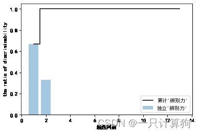
LDA的线性判别数量最多为c-1,c为分类标签的数量
tot=sum(eigen_vals.real)#取实部
discr=[(i/tot) for i in sorted(eigen_vals.real,reverse=True)]
discr
[0.6692795600710417,
 0.3307204399289582,
 2.4247937533367015e-17,
 2.4247937533367015e-17,
 1.4525383988179517e-17,
 0.0,
 -4.3195468201936075e-18,
 -5.582576175728131e-18,
 -5.582576175728131e-18,
 -5.7329513395579316e-18,
 -5.7329513395579316e-18,
 -4.053373328884912e-17,
 -7.246292542455223e-17]
cum_discar=np.cumsum(discr)
辨别力:类的判别信息
#coding:utf-8
import matplotlib.pyplot as plt
plt.rcParams['font.sans-serif']=['SimHei'] #用来正常显示中文标签
plt.rcParams['axes.unicode_minus']=False #用来正常显示负号
#有中文出现的情况,需要u'内容

plt.bar(range(1,14),discr,alpha=0.4,align='center',
       label="独立'辨别力'")
plt.step(range(1,14),cum_discar,where='mid',
        label="累计'辨别力'",color='k')
plt.xlabel('线性判别')
plt.ylabel('the ratio of discriminability')
plt.legend(loc='best')
plt.show()
eigen_pairs[0][1][:,np.newaxis].real
array([[-0.1481],
       [ 0.0908],
       [-0.0168],
       [ 0.1484],
       [-0.0163],
       [ 0.1913],
       [-0.7338],
       [-0.075 ],
       [ 0.0018],
       [ 0.294 ],
       [-0.0328],
       [-0.3547],
       [-0.3915]])
W=np.hstack((eigen_pairs[0][1][:,np.newaxis].real,
             eigen_pairs[1][1][:,np.newaxis].real))
print('matrix W:\n',W)
matrix W:
 [[-0.1481 -0.4092]
 [ 0.0908 -0.1577]
 [-0.0168 -0.3537]
 [ 0.1484  0.3223]
 [-0.0163 -0.0817]
 [ 0.1913  0.0842]
 [-0.7338  0.2823]
 [-0.075  -0.0102]
 [ 0.0018  0.0907]
 [ 0.294  -0.2152]
 [-0.0328  0.2747]
 [-0.3547 -0.0124]
 [-0.3915 -0.5958]]
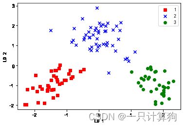
将样本投射到新的特征空间
X ′ = X W X^{'}=XW X′=XW
X_train_lda=X_train_std.dot(W)
colors=['r','b','g']
markers=['s','x','o']
for l,c,m in zip(np.unique(y_train),colors,markers):
    plt.scatter(X_train_lda[y_train==l,0],
                X_train_lda[y_train==l,1],c=c,label=l,
               marker=m)
plt.xlabel('LD 1')
plt.ylabel('LD 2')
plt.legend(loc='best')
plt.show()
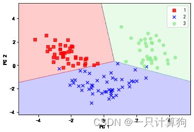
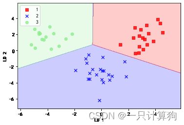
sklearn实现LDA
from sklearn.discriminant_analysis import LinearDiscriminantAnalysis as LDA
lda=LDA(n_components=2)#3个类别
X_train_lda=lda.fit_transform(X_train_std,y_train)#获得投影后新的特征
#使用逻辑斯蒂回归处理低位数据
lr=LogisticRegression(C=1.1)
lr=lr.fit(X_train_lda,y_train)
plot_decision_regions(X_train_lda,y_train,classifier=lr)
plt.xlabel('LD 1')
plt.ylabel('LD 2')
plt.legend(loc='best')
plt.xlim([-3,4])
plt.show()
*c* argument looks like a single numeric RGB or RGBA sequence, which should be avoided as value-mapping will have precedence in case its length matches with *x* & *y*.  Please use the *color* keyword-argument or provide a 2-D array with a single row if you intend to specify the same RGB or RGBA value for all points.
*c* argument looks like a single numeric RGB or RGBA sequence, which should be avoided as value-mapping will have precedence in case its length matches with *x* & *y*.  Please use the *color* keyword-argument or provide a 2-D array with a single row if you intend to specify the same RGB or RGBA value for all points.
*c* argument looks like a single numeric RGB or RGBA sequence, which should be avoided as value-mapping will have precedence in case its length matches with *x* & *y*.  Please use the *color* keyword-argument or provide a 2-D array with a single row if you intend to specify the same RGB or RGBA value for all points.

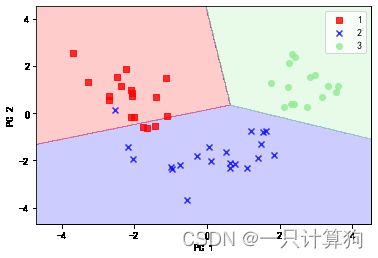
X_test_lda=lda.transform(X_test_std)
plot_decision_regions(X_test_lda,y_test,classifier=lr)
plt.xlabel('LD 1')
plt.ylabel('LD 2')
plt.legend(loc='best')
plt.show()
*c* argument looks like a single numeric RGB or RGBA sequence, which should be avoided as value-mapping will have precedence in case its length matches with *x* & *y*.  Please use the *color* keyword-argument or provide a 2-D array with a single row if you intend to specify the same RGB or RGBA value for all points.
*c* argument looks like a single numeric RGB or RGBA sequence, which should be avoided as value-mapping will have precedence in case its length matches with *x* & *y*.  Please use the *color* keyword-argument or provide a 2-D array with a single row if you intend to specify the same RGB or RGBA value for all points.
*c* argument looks like a single numeric RGB or RGBA sequence, which should be avoided as value-mapping will have precedence in case its length matches with *x* & *y*.  Please use the *color* keyword-argument or provide a 2-D array with a single row if you intend to specify the same RGB or RGBA value for all points.
5.3 KPCA
5.3.2python实现
from scipy.spatial.distance import pdist,squareform
from scipy import exp
from scipy.linalg import eigh
import numpy as np
def rbf_kernel_pca(X,gamma,n_components):

    """
    X:{numpy ndarry},shape={n_samples,n_features}

    gamma: RBF kernel 参数

    n_components:返回的主分空间
    ___________

    returns:
    X_pc:shape=[n_samples,k_features]

    """

    #计算数据集中x之间的平方欧几里得距离
    sq_dists=pdist(X,'sqeuclidean')

    #将距离转化为方阵
    mat_sq_dists=squareform(sq_dists)

    #计算高斯核矩阵
    K=exp(-gamma*mat_sq_dists)

    #中心化核矩阵
    N=K.shape[0]
    one_n=np.ones((N,N)) / N
    K=K-one_n.dot(K)-K.dot(one_n)+one_n.dot(K).dot(one_n)

    #计算中心化核矩阵的特征向量和特征值
    #scipy.linalg.eigh返回降序排列
    eigvals,eigvecs=eigh(K)#特征值按升序排列

    eigvals,eigvecs=eigvals[::-1],eigvecs[:,::-1]#倒着取

    #选择靠前的k个特征向量
    X_pc=np.vstack([eigvecs[:,i] for i in range(n_components)]).T


    return X_pc
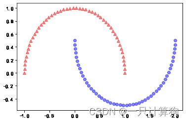
#分离半月形
from sklearn.datasets import make_moons
X,y=make_moons(n_samples=100,random_state=123)
plt.scatter(X[y==0,0],X[y==0,1],
           color='red',marker='^',alpha=0.5)
plt.scatter(X[y==1,0],X[y==1,1],
           color='blue',marker='o',alpha=0.5)
plt.show()
X.shape
(100, 2)
y
array([0, 1, 1, 0, 1, 0, 0, 1, 1, 0, 0, 1, 1, 1, 0, 0, 1, 0, 1, 1, 0, 1,
       0, 0, 0, 1, 1, 0, 1, 0, 0, 1, 0, 1, 1, 1, 1, 1, 1, 0, 0, 1, 0, 1,
       0, 1, 0, 1, 0, 1, 0, 0, 1, 0, 0, 1, 0, 0, 1, 0, 0, 1, 0, 0, 0, 0,
       1, 1, 1, 0, 0, 0, 0, 1, 0, 0, 1, 1, 1, 0, 0, 1, 1, 0, 1, 1, 0, 1,
       1, 0, 0, 0, 1, 0, 1, 1, 1, 0, 1, 1], dtype=int64)
#通过标准的PCA处理
from sklearn.decomposition import PCA
scikit_pca=PCA(n_components=2)
X_spca=scikit_pca.fit_transform(X)

fig,ax=plt.subplots(nrows=1,ncols=2,figsize=(7,3))
ax[0].scatter(X_spca[y==0,0],X_spca[y==0,1],
             color='r',marker='^',alpha=0.5)
ax[0].scatter(X_spca[y==1,0],X_spca[y==1,1],
             color='b',marker='o',alpha=0.5)

ax[0].set_xlabel('PC 1')
ax[0].set_ylabel('PC 2')
ax[0].set_ylim([-1,1])

ax[1].scatter(X_spca[y==0,0],np.zeros((50,1))+0.02,
             color='r',marker='^',alpha=0.5)
ax[1].scatter(X_spca[y==1,0],np.zeros((50,1))+0.02,
             color='b',marker='o',alpha=0.5)
ax[1].set_yticks([])
ax[1].set_xlabel('PC 1')
Text(0.5, 0, 'PC 1')

左图:PCA处理后只是翻转,依然线性不可分
右图:PCA处理后在一维上依然重合
#使用RBF核PCA

X_kpca=rbf_kernel_pca(X,gamma=15,n_components=2)

X_kpca.shape
:23: DeprecationWarning: scipy.exp is deprecated and will be removed in SciPy 2.0.0, use numpy.exp instead
  K=exp(-gamma*mat_sq_dists)


(100, 2)
fig,ax=plt.subplots(nrows=1,ncols=2,figsize=(7,3))
ax[0].scatter(X_kpca[y==0,0],X_kpca[y==0,1],
             color='r',marker='^',alpha=0.5)
ax[0].scatter(X_kpca[y==1,0],X_kpca[y==1,1],
             color='b',marker='o',alpha=0.5)
ax[0].set_xlabel('PC 1')
ax[0].set_ylabel('PC 2')


ax[1].scatter(X_kpca[y==0,0],np.zeros((50,1))+0.02,
             color='r',marker='^',alpha=0.5)
ax[1].scatter(X_kpca[y==1,0],np.zeros((50,1))+0.02,
             color='b',marker='o',alpha=0.5)
ax[1].set_yticks([])
plt.show()

分离同心圆
from sklearn.datasets import make_circles
X,y=make_circles(n_samples=1000,random_state=123,
                noise=0.1,factor=0.2)
X.shape, y.shape
((1000, 2), (1000,))
plt.scatter(X[y==0,0],X[y==0,1],
           color='r',marker='^',alpha=0.5)
plt.scatter(X[y==1,0],X[y==1,1],
           color='b',marker='o',alpha=0.5)

]
#使用标准pca
scikit_pca=PCA(n_components=2)
X_spca=scikit_pca.fit_transform(X)

fig,ax=plt.subplots(nrows=1,ncols=2,figsize=(7,3))
ax[0].scatter(X_spca[y==0,0],X_spca[y==0,1],
             color='r',marker='^',alpha=0.5)
ax[0].scatter(X_spca[y==1,0],X_spca[y==1,1],
             color='b',marker='o',alpha=0.5)
ax[0].set_xlabel('PC 1')
ax[0].set_ylabel('PC 2')


ax[1].scatter(X_spca[y==0,0],np.zeros((500,1))+0.02,
             color='r',marker='^',alpha=0.5)
ax[1].scatter(X_spca[y==1,0],np.zeros((500,1))+0.02,
             color='b',marker='o',alpha=0.5)
ax[1].set_yticks([])
plt.show()

显然PCA不能将数据分开
#使用KPCA
X_kpca=rbf_kernel_pca(X,gamma=15,n_components=2)

fig,ax=plt.subplots(nrows=1,ncols=2,figsize=(7,3))
ax[0].scatter(X_kpca[y==0,0],X_kpca[y==0,1],
             color='r',marker='^',alpha=0.5)
ax[0].scatter(X_kpca[y==1,0],X_kpca[y==1,1],
             color='b',marker='o',alpha=0.5)
ax[0].set_xlabel('PC 1')
ax[0].set_ylabel('PC 2')


ax[1].scatter(X_kpca[y==0,0],np.zeros((500,1))+0.02,
             color='r',marker='^',alpha=0.5)
ax[1].scatter(X_kpca[y==1,0],np.zeros((500,1))+0.02,
             color='b',marker='o',alpha=0.5)
ax[1].set_yticks([])
plt.show()
:23: DeprecationWarning: scipy.exp is deprecated and will be removed in SciPy 2.0.0, use numpy.exp instead
  K=exp(-gamma*mat_sq_dists)

KPCA将数据分开
5.3.3投影新的数据点
def rbf_kernel_pca(X,gamma,n_components):

    """
    X:{numpy ndarry},shape={n_samples,n_features}

    gamma: RBF kernel 参数

    n_components:返回的主分空间
    ___________

    returns:
    X_pc:shape=[n_samples,k_features]

    """

    #计算数据集中x之间的平方欧几里得距离
    sq_dists=pdist(X,'sqeuclidean')

    #将距离转化为方阵
    mat_sq_dists=squareform(sq_dists)

    #计算高斯核矩阵
    K=exp(-gamma*mat_sq_dists)

    #中心化核矩阵
    N=K.shape[0]
    one_n=np.ones((N,N)) / N
    K=K-one_n.dot(K)-K.dot(one_n)+one_n.dot(K).dot(one_n)

    #计算中心化核矩阵的特征向量和特征值
    #scipy.linalg.eigh返回降序排列
    eigvals,eigvecs=eigh(K)#特征值按升序排列

    eigvals,eigvecs=eigvals[::-1],eigvecs[:,::-1]#倒着取

    #选择靠前的k个特征向量
    alphas=np.vstack([eigvecs[:,i] for i in range(n_components)]).T

    #选择特征值
    lambdas=[eigvals[i] for i in range(n_components)]

    return alphas,lambdas
#创建新的半月数据集
X,y=make_moons(n_samples=100,random_state=123)
#RBF核PCA投影到一维数据集
alphas,lambdas=rbf_kernel_pca(X,gamma=15,n_components=1)
:23: DeprecationWarning: scipy.exp is deprecated and will be removed in SciPy 2.0.0, use numpy.exp instead
  K=exp(-gamma*mat_sq_dists)
alphas.shape
(100, 1)
#将第26个数据点投射到新的子空间
x_new=X[25]
x_new
array([1.8713, 0.0093])
x_proj=alphas[25]
x_proj
array([0.0788])
def project_x(x_new,X,gamma,alphas,lambdas):
    pair_dist=np.array([np.sum((x_new-row)**2 ) for row in X])
    k=np.exp(-gamma*pair_dist)
    return k.dot(alphas/lambdas)
#验证
x_reproj=project_x(x_new,X,gamma=15.0,alphas=alphas,lambdas=lambdas)
x_reproj
array([0.0788])
#coding:utf-8
import matplotlib.pyplot as plt
plt.rcParams['font.sans-serif']=['SimHei'] #用来正常显示中文标签
plt.rcParams['axes.unicode_minus']=False #用来正常显示负号
#有中文出现的情况,需要u'内容


#投影可视化
plt.scatter(alphas[y==0,0],np.zeros((50)),
           color='r',marker='^',alpha=0.5)
plt.scatter(alphas[y==1,0],np.zeros(50),
           color='b',marker='o',alpha=0.5)
plt.scatter(x_proj,0,color='black',
           label='X[25]的原始投影',marker='^',s=100)
plt.scatter(x_reproj,0,color='g',
           label='重新投影的点X[25]',marker='x',s=500)
plt.legend(loc='best')
plt.show()

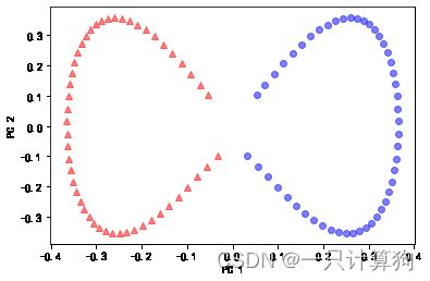
5.3.4 sklearn实现核主成分分析
from sklearn.decomposition import KernelPCA
X,y=make_moons(n_samples=100,random_state=123)
sklearn_kpca=KernelPCA(n_components=2,kernel='rbf',gamma=15)
X_skernpac=sklearn_kpca.fit_transform(X)
plt.scatter(X_skernpac[y==0,0],X_skernpac[y==0,1],
           color='r',marker='^',alpha=0.5)
plt.scatter(X_skernpac[y==1,0],X_skernpac[y==1,1],
           color='b',marker='o',alpha=0.5)
plt.xlabel('PC 1')
plt.ylabel('PC 2')
Text(0, 0.5, 'PC 2')