学习笔记 | Python处理矢栅数据(1)
文章目录
- 1. 栅格数据介绍
- 2. 栅格数据重投影
- 3. 栅格计算
- 4. 栅格重分类
- 5. 设置元数据并到处为GeoTiff
1. 栅格数据介绍

import rioxarray
import matplotlib
sr_HARV = rioxarray.open_rasterio("G:/learnpy/data/NEOSAirRS/HARV/DSM/HARV_dsmCrop.tif")
sr_HARV

print(sr_HARV.rio.crs)
print(sr_HARV.rio.nodata)
print(sr_HARV.rio.bounds())
print(sr_HARV.rio.resolution())
print(sr_HARV.rio.width)
print(sr_HARV.rio.height)
print(sr_HARV.values)

# 输出
EPSG:32618
-9999.0
(731453.0, 4712471.0, 733150.0, 4713838.0)
(1.0, -1.0)
1697
1367
[[[408.76998901 408.22998047 406.52999878 ... 345.05999756 345.13998413
   344.97000122]
  [407.04998779 406.61999512 404.97998047 ... 345.20999146 344.97000122
   345.13998413]
  [407.05999756 406.02999878 403.54998779 ... 345.07000732 345.08999634
   345.17999268]
  ...
  [367.91000366 370.19000244 370.58999634 ... 311.38998413 310.44998169
   309.38998413]
  [370.75997925 371.50997925 363.41000366 ... 314.70999146 309.25
   312.01998901]
  [369.95999146 372.6000061  372.42999268 ... 316.38998413 309.86999512
   311.20999146]]]
sr_HARV.plot()

print(sr_HARV.rio.crs)
print(sr_HARV.rio.crs.to_epsg())
# EPSG:32618
# 32618
from pyproj import CRS
epsg = sr_HARV.rio.crs.to_epsg()
epsg
# 32618
crs = CRS(epsg)
crs
##############################
#print(crs.name)
crs.area_of_use
###################
# WGS 84 / UTM zone 18N
# AreaOfUse(west=-78.0, south=0.0, east=-72.0, north=84.0, name='Between 78°W and 72°W, northern hemisphere between equator and 84°N, onshore and offshore. Bahamas. Canada - Nunavut; Ontario; Quebec. Colombia. Cuba. Ecuador. Greenland. Haiti. Jamica. Panama. Turks and Caicos Islands. United States (USA). Venezuela.')
# 求最大值、最小值、均值、标准差
print(sr_HARV.max())
print(sr_HARV.min())
print(sr_HARV.mean())
print(sr_HARV.std())

######################
<xarray.DataArray ()>
array(416.06997681)
Coordinates:
    spatial_ref  int32 0
<xarray.DataArray ()>
array(305.07000732)
Coordinates:
    spatial_ref  int32 0
<xarray.DataArray ()>
array(359.85311803)
Coordinates:
    spatial_ref  int32 0
<xarray.DataArray ()>
array(17.83168952)
Coordinates:
    spatial_ref  int32 0
print(sr_HARV.quantile([0.25,0.75]))
####################################
<xarray.DataArray (quantile: 2)>
array([345.58999634, 374.27999878])
Coordinates:
  * quantile  (quantile) float64 0.25 0.75
# 也可以通过numpy来得到这些值
import numpy as np
print(np.percentile(sr_HARV,25))
print(np.percentile(sr_HARV,75))
# 345.5899963378906
# 374.2799987792969
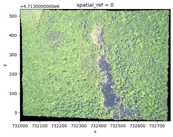
rgb_HARV = rioxarray.open_rasterio("G:/learnpy/data/NEOSAirRS/HARV/RGB_Imagery/HARV_RGB_Ortho.tif")
rgb_HARV
###################
<xarray.DataArray (band: 3, y: 2317, x: 3073)>
[21360423 values with dtype=float64]
Coordinates:
  * band         (band) int32 1 2 3
  * x            (x) float64 7.32e+05 7.32e+05 7.32e+05 ... 7.328e+05 7.328e+05
  * y            (y) float64 4.714e+06 4.714e+06 ... 4.713e+06 4.713e+06
    spatial_ref  int32 0
Attributes:
    STATISTICS_MAXIMUM:  255
    STATISTICS_MEAN:     nan
    STATISTICS_MINIMUM:  0
    STATISTICS_STDDEV:   nan
    _FillValue:          -1.7e+308
    scale_factor:        1.0
    add_offset:          0.0
rgb_HARV.plot.imshow(robust=True)
2. 栅格数据重投影
DTMhill_HARV.rio.reproject_match
DTMhill_HARV.rio.reproject_match
import rioxarray
import matplotlib
surface_HARV = rioxarray.open_rasterio("G:/learnpy/data/NEOSAirRS/HARV/DSM/HARV_dsmCrop.tif")
terrain_HARV = rioxarray.open_rasterio("G:/learnpy/data/NEOSAirRS/HARV/DTM/HARV_dtmCrop.tif")
DTMhill_HARV = rioxarray.open_rasterio("G:/learnpy/data/NEOSAirRS/HARV/DTM/HARV_DTMhill_WGS84.tif")
surface_HARV

######################
<xarray.DataArray (band: 1, y: 1367, x: 1697)>
[2319799 values with dtype=float64]
Coordinates:
  * band         (band) int32 1
  * x            (x) float64 7.315e+05 7.315e+05 ... 7.331e+05 7.331e+05
  * y            (y) float64 4.714e+06 4.714e+06 ... 4.712e+06 4.712e+06
    spatial_ref  int32 0
Attributes:
    STATISTICS_MAXIMUM:  416.06997680664
    STATISTICS_MEAN:     359.85311802914
    STATISTICS_MINIMUM:  305.07000732422
    STATISTICS_STDDEV:   17.83169335933
    _FillValue:          -9999.0
    scale_factor:        1.0
    add_offset:          0.0
surface_HARV.rio.crs.wkt

#########################
# We can see the datum and projection are UTM zone 18N and WGS 84 respectively.
'PROJCS["WGS 84 / UTM zone 18N",GEOGCS["WGS 84",DATUM["WGS_1984",SPHEROID["WGS 84",6378137,298.257223563,AUTHORITY["EPSG","7030"]],AUTHORITY["EPSG","6326"]],PRIMEM["Greenwich",0,AUTHORITY["EPSG","8901"]],UNIT["degree",0.0174532925199433,AUTHORITY["EPSG","9122"]],AUTHORITY["EPSG","4326"]],PROJECTION["Transverse_Mercator"],PARAMETER["latitude_of_origin",0],PARAMETER["central_meridian",-75],PARAMETER["scale_factor",0.9996],PARAMETER["false_easting",500000],PARAMETER["false_northing",0],UNIT["metre",1,AUTHORITY["EPSG","9001"]],AXIS["Easting",EAST],AXIS["Northing",NORTH],AUTHORITY["EPSG","32618"]]'
DTMhill_HARV.rio.crs.wkt
# 'GEOGCS["WGS 84",DATUM["WGS_1984",SPHEROID["WGS 84",6378137,298.257223563,AUTHORITY["EPSG","7030"]],AUTHORITY["EPSG","6326"]],PRIMEM["Greenwich",0],UNIT["degree",0.0174532925199433,AUTHORITY["EPSG","9122"]],AXIS["Latitude",NORTH],AXIS["Longitude",EAST],AUTHORITY["EPSG","4326"]]'
# we can see the DTMhill is in unprojected geographic coodinate system
DTMhill_HARV_pro = DTMhill_HARV.rio.reproject_match(surface_HARV)
DTMhill_HARV_pro.rio.crs.wkt
# 'PROJCS["WGS 84 / UTM zone 18N",GEOGCS["WGS 84",DATUM["WGS_1984",SPHEROID["WGS 84",6378137,298.257223563,AUTHORITY["EPSG","7030"]],AUTHORITY["EPSG","6326"]],PRIMEM["Greenwich",0,AUTHORITY["EPSG","8901"]],UNIT["degree",0.0174532925199433,AUTHORITY["EPSG","9122"]],AUTHORITY["EPSG","4326"]],PROJECTION["Transverse_Mercator"],PARAMETER["latitude_of_origin",0],PARAMETER["central_meridian",-75],PARAMETER["scale_factor",0.9996],PARAMETER["false_easting",500000],PARAMETER["false_northing",0],UNIT["metre",1,AUTHORITY["EPSG","9001"]],AXIS["Easting",EAST],AXIS["Northing",NORTH],AUTHORITY["EPSG","32618"]]'
DTMhill_HARV_pro.rio.to_raster("G:/learnpy/data/NEOSAirRS/HARV/DTM/HARV_DTMhill_WGS84_utm_18.tif")
DTMhill_HARV_pro.plot(cmap = "viridis")
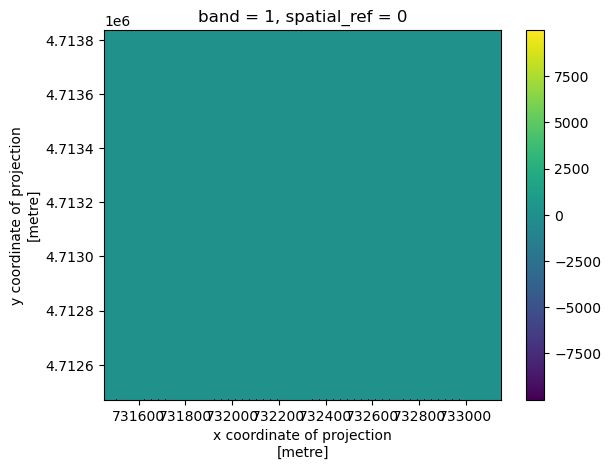
DTMhill_HARV_pro_valid = DTMhill_HARV_pro.where(DTMhill_HARV_pro != DTMhill_HARV_pro.rio.nodata)
DTMhill_HARV_pro_valid.plot(cmap = "viridis")

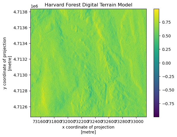
import matplotlib.pyplot as plt
DTMhill_HARV_pro_valid.plot(cmap = "viridis")
plt.title("Harvard Forest Digital Terrain Model")
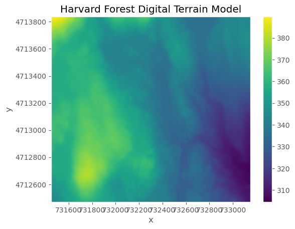
terrain_HARV_valid = terrain_HARV.where(terrain_HARV != terrain_HARV.rio.nodata)
terrain_HARV_valid.plot()
plt.title("Harvard Forest Digital Terrain Model")

plt.style.use("ggplot")
terrain_HARV_valid.plot()
plt.title("Harvard Forest Digital Terrain Model")
plt.ticklabel_format(style="plain")
练习SJER数据,重投影并作图
surface_SJER = rioxarray.open_rasterio("G:/learnpy/data/NEOSAirRS/SJER/DSM/SJER_dsmCrop.tif",masked=True)
terrain_SJER = rioxarray.open_rasterio("G:/learnpy/data/NEOSAirRS/SJER/DTM/SJER_dtmCrop.tif",masked = True)
surface_SJER.plot()

plt.figure()
terrain_SJER.plot()
plt.title("SJER Digital Surface Model")

plt.figure()
surface_SJER.plot()
plt.title("SJER Digital Terrain Model")


3. 栅格计算

surface_SJER = rioxarray.open_rasterio("G:/learnpy/data/NEOSAirRS/SJER/DSM/SJER_dsmCrop.tif",masked=True)
terrain_SJER = rioxarray.open_rasterio("G:/learnpy/data/NEOSAirRS/SJER/DTM/SJER_dtmCrop.tif",masked = True)
surface_SJER.rio.crs.wkt == terrain_SJER.rio.crs.wkt
# True
CHM_SJER = surface_SJER - terrain_SJER
CHM_SJER
#########################
<xarray.DataArray (band: 1, y: 2178, x: 2005)>
array([[[0.1000061 , 0.3999939 , 1.05999756, ..., 0.        ,
         0.        , 0.        ],
        [0.        , 0.        , 1.70999146, ..., 0.        ,
         0.        , 0.        ],
        [0.        , 0.42999268, 1.35998535, ..., 0.        ,
         0.        , 0.        ],
        ...,
        [0.01000977, 0.        , 0.08001709, ..., 1.64001465,
         7.41000366, 0.98999023],
        [0.04998779, 0.        , 0.        , ..., 0.23001099,
         8.63000488, 1.25      ],
        [0.        , 0.        , 0.        , ..., 0.07998657,
         0.19000244, 0.        ]]])
Coordinates:
  * band         (band) int32 1
  * x            (x) float64 2.557e+05 2.557e+05 ... 2.577e+05 2.577e+05
  * y            (y) float64 4.112e+06 4.112e+06 4.112e+06 ... 4.11e+06 4.11e+06
    spatial_ref  int32 0
CHM_SJER.plot(cmap = "viridis")

print(CHM_SJER.max())
print(CHM_SJER.min())

########################
<xarray.DataArray ()>
array(32.63000488)
Coordinates:
    spatial_ref  int32 0
<xarray.DataArray ()>
array(-1.3999939)
Coordinates:
    spatial_ref  int32 0
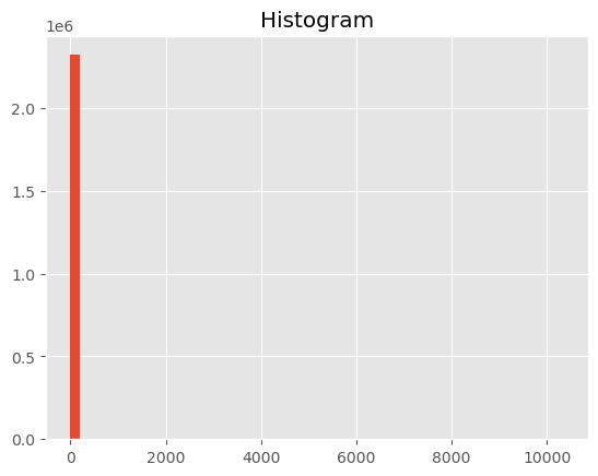
CHM_SJER.plot.hist(bins = 50)

surface_HARV1 = rioxarray.open_rasterio("G:/learnpy/data/NEOSAirRS/HARV/DSM/HARV_dsmCrop.tif",masked=True)#去除了fillValue-9999
print(surface_HARV1)#去除了fillValue-9999

########################################
<xarray.DataArray (band: 1, y: 1367, x: 1697)>
[2319799 values with dtype=float64]
Coordinates:
  * band         (band) int32 1
  * x            (x) float64 7.315e+05 7.315e+05 ... 7.331e+05 7.331e+05
  * y            (y) float64 4.714e+06 4.714e+06 ... 4.712e+06 4.712e+06
    spatial_ref  int32 0
Attributes:
    STATISTICS_MAXIMUM:  416.06997680664
    STATISTICS_MEAN:     359.85311802914
    STATISTICS_MINIMUM:  305.07000732422
    STATISTICS_STDDEV:   17.83169335933
    scale_factor:        1.0
    add_offset:          0.0
terrain_HARV1 = rioxarray.open_rasterio("G:/learnpy/data/NEOSAirRS/HARV/DTM/HARV_dtmCrop.tif",masked=True)
print(terrain_HARV1)
terrain_HARV1.plot.hist(bins=50)

CHM_HARV = surface_HARV - terrain_HARV
print(CHM_HARV.min().values)
print(CHM_HARV.max().values)
CHM_HARV.plot.hist(bins=50)
CHM_HARV1 = surface_HARV1 - terrain_HARV1
CHM_HARV1.plot.hist(bins=50)

4. 栅格重分类
import numpy as np
import rioxarray
# difine the bins for pixel values
class_bins = [CHM_HARV1.min().values, 2, 10, 20, np.inf]
class_bins
# classifies the original canopy height model array
canopy_height_classes = np.digitize(CHM_HARV1, class_bins)
print(type(canopy_height_classes))
canopy_height_classes
#############################################
#import xarray
from matplotlib.colors import ListedColormap
import earthpy.plot as ep
import matplotlib.pyplot as plt
#define color map of the legend
height_colors = ["gray", "y", "yellowgreen", "g", "darkgreen"]
height_cmap = ListedColormap(height_colors)
height_cmap

# define classname for the legend
category_names = [
    "No Vegetation",
    "Bare Area",
    "Low Canopy",
    "Medium Canopy",
    "Tall Canopy",
]
category_names
# ['No Vegetation', 'Bare Area', 'Low Canopy', 'Medium Canopy', 'Tall Canopy']
# we should konw in what order the legend items should be arranged
category_indices = list(range(len(category_names)))
category_indices
# [0, 1, 2, 3, 4]
# we put the numpy array in a xarray DataArray so that the plot is made with coordinates
canopy_height_classified = xarray.DataArray(canopy_height_classes, coords=CHM_HARV1.coords)
canopy_height_classified

############################################
<xarray.DataArray (band: 1, y: 1367, x: 1697)>
array([[[3, 3, 3, ..., 1, 1, 1],
        [3, 3, 3, ..., 1, 1, 1],
        [3, 3, 3, ..., 1, 1, 1],
        ...,
        [4, 4, 4, ..., 1, 1, 1],
        [4, 4, 3, ..., 2, 1, 2],
        [4, 4, 4, ..., 2, 1, 1]]], dtype=int64)
Coordinates:
  * band         (band) int32 1
  * x            (x) float64 7.315e+05 7.315e+05 ... 7.331e+05 7.331e+05
  * y            (y) float64 4.714e+06 4.714e+06 ... 4.712e+06 4.712e+06
    spatial_ref  int32 0
# Making the plot
plt.style.use("default")
plt.figure()
im = canopy_height_classified.plot(cmap = height_cmap, add_colorbar = False)
ep.draw_legend(im_ax=im, classes = category_indices, titles = category_names)
plt.title("Classfied Canopy Heihgt Model-NEON Harvard Forest Field Site")
plt.ticklabel_format(style="plain")

5. 设置元数据并到处为GeoTiff
CHM_HARV1.rio.write_crs(surface_HARV1.rio.crs, inplace=True)
CHM_HARV1.rio.set_nodata(-9999.0, inplace=True)
CHM_HARV1.rio.to_raster("G:/learnpy/data/NEOSAirRS/HARV/CHM_HARV.tif")
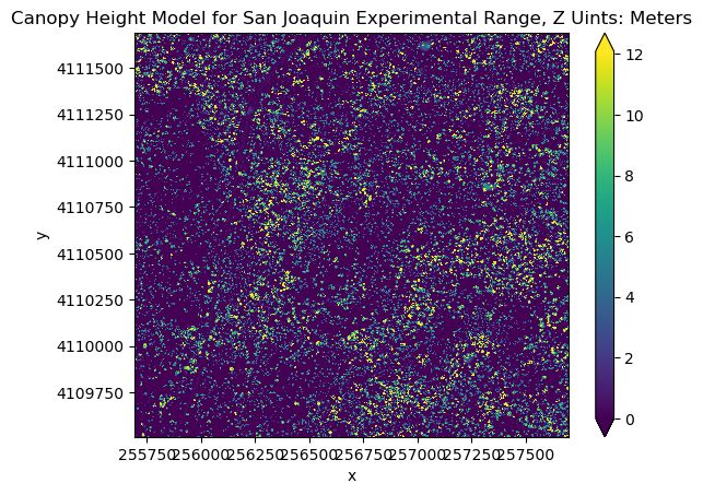
CHM_SJER = surface_SJER - terrain_SJER
plt.figure()
CHM_SJER.plot(robust=True, cmap = "viridis")
plt.ticklabel_format(style = "plain")
plt.title("Canopy Height Model for San Joaquin Experimental Range, Z Uints: Meters")
# Campare the SJER and HARV
fig, ax = plt.subplots(figsize = (9,6))
CHM_HARV1.plot.hist(ax = ax, bins =50, color="green")
CHM_SJER.plot.hist(ax = ax, bins = 50,color="orange")

Tips:
rioxarray
NEON-geopy