机器学习基础以及在pynq-Z2上部署Faster-RCNN的项目学习1
目录
一.python代码基础
1.1.原始数据类型与操作
1.1.1.数值型
1.1.2.布尔型
1.1.3.字符串
1.1.4.其他
1.2.变量与集合
1.2.1.输入输出
1.2.2.列表(List)
1.2.3.元组(Tuple)
1.2.4.字典(Dictionaries)
1.2.5.集合(Set)
1.3.控制流
1.3.1.分支结构
1.3.2.循环结构
1.3.3.异常处理
1.3.4.迭代器
1.3.5.函数
1.3.6.函数的作用域
1.3.7.类
1.3.8.模块
1.3.9.高级
二.机器学习基础(了解与认识)
2.1机器学习的本质
2.2.机器学习的流程和步骤
2.2.1.收集输入与输出的例子
2.2.2.建立模型
2.2.3.确定输入输出与模型可接收返回的数值之间如何转换
2.2.4.使用输入与输出的例子调整模型的参数
2.2.5.使用没有参与训练的输入与输出评价模型是否成功摸索处规律(检验)
2.3.机器学习、深度学习和人工智能的区别
2.4.一个最简单的例子
2.5.机器学习
2.6.让参数调整量依赖于损失的
三.pytorch与矩阵计算入门
3.1.Pytorch简介
3.2.学Pytorch好还是Tensorflow好?
3.2.1.Dynamic Graph 与 Static Graph
3.3.安装Pytorch
3.4.Pytorch
3.5.Pytorch保存tensor使用的数据结构
3.6.矩阵乘法简介
3.7.使用Pytorch进行矩阵乘法计算
3.8.Pytorch的自动微分功能(autograd)
3.9.Pytorch的损失计算器封装(Loss function)
3.10.Pytorch的参数调整器封装(optimizer)
3.11.使用Pytorch实现二中的例子
3.12.使用矩阵乘法实现批次训练
3.13.划分训练集,验证集和测试机的例子
3.14.定义模型类(torch.nn.Module)
四.线性模型,激活函数和多层线性模型
4.1.生物神经元与人工神经元
4.2.单层线性模型
4.3.激活函数
4.4.多层线性模型
4.5.根据码农条件求工资
一.python代码基础
1.1.原始数据类型与操作
1.1.1.数值型
# 数值型
3 # => 3

# 数学计算
1 + 1 # => 2
8 - 1 # => 7
10 * 2 # => 20
35 / 5 # => 7

# 整型(int)的除法只会获得整型结果,余数自动舍弃 Python 2.7
5 / 2 # => 2
# Python会自动返回浮点数
5 / 2 # => 2.5

# 浮点型(float)的计算可以有小数
2.0 # 这是一个浮点型
11.0 / 4.0 # => 2.75

# 如果只需要整数部分,使用"//"做除法,又叫地板除(foored division)
5 // 3 # => 1
5.0 // 3.0 # => 1.0 浮点型效果也一样
-5 // 3 # => -2
-5.0 // 3.0 # => -2.0

# 取余操作
7 % 3 # => 1

# 幂操作
2 ** 4 # => 16

# 使用括号改变优先级
(1+3) * 2 # => 8
1.1.2.布尔型
# 注: "and" 和 "or" 都是大小写敏感的
True and False # => False
False or True # => True

# 注:int型也可以使用布尔操作
0 and 2 # => 0
-5 or 0 # => -5
0 == False # => True
2 == True # => False
1 == True # => True

# 非操作
not True # => False
not False # => True

# 判断相等
1 == 1 # => True
2 == 1 # => False

# 判断不相等
1 != 1 # => False
2 != 1 # => True

# 其它比较操作
1 < 10 # => True
1 > 10 # => False
2 <= 2 # => True
2 >= 2 # => True

# 比较操作可以串联
1 < 2 < 3 # => True
1 < 3 < 2 # => False

# is 与 == 比较
# is 是判断两个变量是否引用了同一个类
# == 是判断两个变量是否有同样的值
a = [1, 2, 3, 4]  # 将 a 指向一个新的数组 [1, 2, 3, 4]
b = a             # 将 b 指向 a 所指向的对象
b is a            # => True, a 和 b 引用了同一个对象
b == a            # => True, a 和 b 的对象值也相同
b = [1, 2, 3, 4]  # 将 b 指向一个新的数组 [1, 2, 3, 4]
b is a            # => False, a 和 b 不是引用了同一个对象
b == a            # => True, a 和 b 的对象值相同
1.1.3.字符串
# 字符串使用 单引号 或者 双引号 表示
"这是一个字符串"
'这也是一个字符串'

# 字符串可以使用"+"连接
"Hello " + "world!" # "Hello world!"
# 不使用"+"也可以让字符串连接
"Hello " "world!" # "Hello world!"

# 字符串乘法
"Hello" * 3 # => "HelloHelloHello"

# 字符串可以当作字符数组操作
"This is a string"[0] # => "T"

# 使用 % 对字符串进行格式化
# 从Python 3.1 开始已经不推荐使用了,但了解一下如何使用还是有必要的
x = 'apple'
y = 'lemon'
z = "The items in the basket are %s and %s " % (x,y)

# 新的格式化字符串的方式是使用format方法
"{} is a {}".format("This", "placeholder")
"{0} can be {1}".format("strings", "formatted")
# 如果不想用下标方式,可以使用关键字的方式
"{name} wants to eat {food}".format(name="Bob", food="lasagna")
1.1.4.其他
# None 是一个对象
None # => None

# 如果想要将一个对象与None进行比较,使用 is 而不要使用 == 符号
"etc" is None # => False
None is None # => True

# is 操作用来判断对象的类型。在对象操作时非常有用

# 任何一个对象都可以放在一个布尔上下文中进行判断
# 下面的情况会被当作False
#   - None
#   - 值为0的任何数值类型,(例如,0,0L,0.0,0j)
#   - 空列表,(例如,'',(),[])
#   - 空的容器,(例如,{},set())
#   - 符合条件的用户自定义对象实例,参看:https://docs.python.org/2/reference/datamodel.html#object.__nonzero__
#
# 其它情况下的值会被当作True,可以使用bool()函数来判断
bool(0)   # => False
bool("")  # => False
bool([])  # => False
bool({})  # => False
1.2.变量与集合
1.2.1.输入输出
# Python有一个打印语句
print "I'm Python. Nice to meet you!" # => I'm Python. Nice to meet you!

# 获取控制台输入的简单方法
input_string_var = raw_input("Enter some data: ") # 返回字符串类型的数据
input_var = input("Enter some data: ") # 返回数值型的数据
# Warning: Caution is recommended for input() method usage
# 注意:在Python3中,input()已经不再使用,raw_input()重命名为input()

# 不需要先声明变量再使用
some_var = 5    # 通常使用小写字母与下划线命名变量
some_var  # => 5

# 访问一个未定义的变量会抛出一个异常
# 在“控制流”里会介绍更多异常处理
some_other_var  # 这里会抛出一个NameError

# if 可以用来写成类似C语言的 '?:' 条件表达式
"yahoo!" if 3 > 2 else 2  # => "yahoo!"
1.2.2.列表(List)
# List用来存储列表
li = []
# 可以有初始数据
other_li = [4, 5, 6]

# 添加元素到列表的尾
li.append(1) # [1]
li.append(2) # [1,2]
li.append(4) # [1,2,4]
li.append(3) # [1,2,4,3]
# 使用pop方法移除列表末尾的元素
li.pop()        # => 3 列表现在为 [1, 2, 4]
# 把3再放回去
li.append(3)    # li 现在为 [1, 2, 4, 3]

# 像数组一样访问一个list
li[0]  # => 1
# 通过下标重新定义一个元素的值
li[0] = 42
li[0]  # => 42
li[0] = 1  # 注意:设置回原始值
# 查看最后一个元素
li[-1]  # => 3

# 查找超过数据长度的值会抛出异常: IndexError
li[4]  # 抛出 IndexError

# 可以使用切片句法访问列表
# 这里类型数学上的开/闭区间
li[1:3]  # => [2, 4]
li[2:]  # => [4, 3]
li[:3]  # => [1, 2, 4]
li[::2]   # =>[1, 4]
li[::-1]   # => [3, 4, 2, 1]
# 使用高级切片句法
# li[start:end:step]

# 使用切片进行深层拷贝
li2 = li[:]  # => li2 = [1, 2, 4, 3] 但 (li2 is li) 返回 false


# 使用“del”直接从列表中删除元素
del li[2] #liisnow[1,2,3]

# 可以直接添加一个列表
li+other_li #=>[1,2,3,4,5,6]
# 注: 变量li 和 other_li 值并没有变化

# 使用extend()方法,把列表串起来
li.extend(other_li)   # Now li is [1, 2, 3, 4, 5, 6]

# 删除第一个值与参数相同的元素
li.remove(2)  # li is now [1, 3, 4, 5, 6]
li.remove(2)  # 抛出异常 ValueError 列表中没有2

# 在指定下标插入元素
li.insert(1, 2)  # li is now [1, 2, 3, 4, 5, 6] again

# 获得第一个匹配的元素的下标
li.index(2)  # => 1
li.index(7)  # 抛出异常 ValueError 列表中没有7

# 使用“in”来检查列表中是否包含元素
1 in li #=>True
# 使用“len()”来检查列表的长度
len(li)   # => 6
1.2.3.元组(Tuple)
# 元组(Tuple)与列表类似但不可修改
tup = (1, 2, 3)
tup[0]   # => 1
tup[0] = 3  # 抛出异常 TypeError

# 注意:如果一个元组里只有一个元素,则需要在元素之后加一个逗号;如果元组里没有元素,反而不用加逗号
type((1))   # =>
type((1,))  # =>
type(())    # =>

# 以下对列表的操作,也可以用在元组上
len(tup) # => 3
tup+(4,5,6) #=>(1,2,3,4,5,6)
tup[:2] #=>(1,2)
2intup #=>True

# 可以把元组的值分解到多个变量上
a,b,c= (1, 2, 3) #a is now 1,b  is now 2 and c is now 3
d,e,f= 4,5,6 # 也可以不带括号
# 如果不带括号,元组会默认带上
g = 4, 5, 6 #=>(4,5,6)
# 非常容易实现交换两个变量的值
e, d = d, e # d is now 5 and e is now 4
1.2.4.字典(Dictionaries)
# 字典用来存储(键-值)映射关系
empty_dict = {}
# 这里有个带初始值的字典
filled_dict = {"one": 1, "two": 2, "three": 3}

# 注意:字典 key 必须是不可以修改类型,以确保键值可以被哈希后进行快速检索
# 不可修改的类型包括:int, float, string, tuple
invalid_dict = {[1,2,3]: "123"}  # => Raises a TypeError: unhashable type: 'list'
valid_dict = {(1,2,3):[1,2,3]}   # Values can be of any type, however.

# 使用[]查找一个元素
filled_dict["one"]   # => 1
# 使用"keys()"获得所有的“键”
filled_dict.keys()   # => ["three", "two", "one"]
# 注:字典的key是无序的,结果可以不匹配
# 使用"values()"获得所有的“值”
filled_dict.values()   # => [3, 2, 1]
# 注:同样,这是无序的
# 查询字条中是否存在某个”键“用 "in"
"one" in filled_dict   # => True
1 in filled_dict   # => False
# 查找一个不存在的key会抛出异常 KeyError
filled_dict["four"]   # KeyError
# 使用 "get()" 会避免抛出异常 KeyError
filled_dict.get("one") # => 1
filled_dict.get("four") # => None
# get方法支持默认参数,当key不存在时返回该默认参数
filled_dict.get("one", 4) #=>1
filled_dict.get("four", 4)   # => 4
# 注 filled_dict.get("four") 仍然返回 None
# (get不会把值插入字典中)
# 向字典中插入值的方式与list相同
filled_dict["four"] = 4  # now, filled_dict["four"] => 4
# "setdefault()" 只有首次插入时才会生效
filled_dict.setdefault("five", 5)  # filled_dict["five"] is set to 5
filled_dict.setdefault("five", 6)  # filled_dict["five"] is still 5

# 使用 del 从字典中删除一个键
del filled_dict["one"]  # Removes the key "one" from filled dict

# 从 Python 3.5 开始,可以使用**操作
{'a': 1, **{'b': 2}}  # => {'a': 1, 'b': 2}
{'a': 1, **{'a': 2}}  # => {'a': 2}
1.2.5.集合(Set)
# Set与list类似,但不存储重复的元素
empty_set = set()
some_set = set([1, 2, 2, 3, 4])   # some_set is now set([1, 2, 3, 4])

# 与字典类型一样,Set 里的元素也必须是不可修改的
invalid_set = {[1], 1}  # => Raises a TypeError: unhashable type: 'list'
valid_set = {(1,), 1}

# Set也是无序的,尽管有时看上去像有序的
another_set = set([4, 3, 2, 2, 1])  # another_set is now set([1, 2, 3, 4])
# 从Python 2.7开妈, {}可以用来声明一个Set
filled_set={1,2,2,3,4} #=>{1,2,3,4}
# Can set new variables to a set
filled_set = some_set
# 向Set中添加元素
filled_set.add(5)   # filled_set is now {1, 2, 3, 4, 5}
# 用 & 求 Set的交集
other_set = {3, 4, 5, 6}
filled_set & other_set # =>{3,4,5}
# 用 | 求 Set的合集
filled_set | other_set # =>{1,2,3,4,5,6}
# Do set difference with -
{1,2,3,4}-{2,3,5} # => {1,4}
# Do set symmetric difference with ^
{1,2,3,4}^{2,3,5} #=>{1,4,5}
# 检查右边是否是左边的子集
{1, 2} >= {1, 2, 3} # => False
# 检查左边是否是右边的子集
{1, 2} <= {1, 2, 3} # => True
# 检查元素是否在集合中
2 in filled_set   # => True
10 in filled_set   # => False
1.3.控制流
1.3.1.分支结构
# 先定义一个变量
some_var = 5
# 这里用到了if语句 缩进是Python里的重要属性
# 打印 "some_var is smaller than 10"
if some_var > 10:
    print "some_var is totally bigger than 10."
elif some_var < 10:    # This elif clause is optional.
    print "some_var is smaller than 10."
else:           # This is optional too.
    print "some_var is indeed 10."
1.3.2.循环结构
# For 循环用来遍历一个列表
for animal in ["dog", "cat", "mouse"]:
    # 使用{0}格式 插入字符串
    print "{0} is a mammal".format(animal)

# "range(number)" 返回一个包含数字的列表
for i in range(4):
print i

# "range(lower, upper)" 返回一个从lower数值到upper数值的列表
for i in range(4, 8):
print i

# "range(lower, upper, step)" 返回一个从lower数值到upper步长为step数值的列表
# step 的默认值为1
for i in range(4, 8, 2):
    print(i)
# While 循环会一致执行下去,直到条件不满足
x=0
while x < 4:
print x
x+=1 #x=x+1的简写1.3.3.异常处理
# 使用 try/except 代码块来处理异常
# 自 Python 2.6 以上版本支持:
try:
    # 使用 "raise" 来抛出一个异常
    raise IndexError("This is an index error")
except IndexError as e:
    pass    # Pass 表示无操作. 通常这里需要解决异常.
except (TypeError, NameError):
    pass    # 如果需要多个异常可以同时捕获
else:   # 可选项. 必须在所有的except之后
    print "All good!"   # 当try语句块中没有抛出异常才会执行
finally: #  所有情况都会执行
    print "We can clean up resources here"

# with 语句用来替代 try/finally 简化代码
with open("myfile.txt") as f:
    for line in f:
        print line
1.3.4.迭代器
# Python offers a fundamental abstraction called the Iterable.
# An iterable is an object that can be treated as a sequence.
# The object returned the range function, is an iterable.

filled_dict = {"one": 1, "two": 2, "three": 3}
our_iterable = filled_dict.keys()
print(our_iterable)  # => dict_keys(['one', 'two', 'three']). This is an object that implements our Iterable interface.

# We can loop over it.
for i in our_iterable:
    print(i)  # Prints one, two, three

# However we cannot address elements by index.
our_iterable[1]  # Raises a TypeError

# An iterable is an object that knows how to create an iterator.
our_iterator = iter(our_iterable)

# Our iterator is an object that can remember the state as we traverse through it.
# We get the next object with "next()".
next(our_iterator)  # => "one"

# It maintains state as we iterate.
next(our_iterator)  # => "two"
next(our_iterator)  # => "three"

# After the iterator has returned all of its data, it gives you a StopIterator Exception
next(our_iterator)  # Raises StopIteration

# You can grab all the elements of an iterator by calling list() on it.
list(filled_dict.keys())  # => Returns ["one", "two", "three"]
1.3.5.函数
# 使用 "def" 来创建一个新的函数
def add(x, y):
    print "x is {0} and y is {1}".format(x, y)
    return x + y    # 用 return 语句返回值
# 调用函数
add(5,6) #=>prints out "x is 5 and y is 6" 返回值为11
# 使用关键字参数调用函数
add(y=6, x=5)   # 关键字参数可以不在乎参数的顺序
# 函数的参数个数可以不定,使用*号会将参数当作元组
def varargs(*args):
    return args
varargs(1, 2, 3)   # => (1, 2, 3)

# 也可以使用**号将参数当作字典类型
def keyword_args(**kwargs):
    return kwargs
  # 调用一下试试看
keyword_args(big="foot", loch="ness") # => {"big": "foot", "loch": "ness"}

# 两种类型的参数可以同时使用
def all_the_args(*args, **kwargs):
    print args
    print kwargs
"""
all_the_args(1, 2, a=3, b=4) prints:
    (1, 2)
    {"a": 3, "b": 4}
"""

# When calling functions, you can do the opposite of args/kwargs!
# Use * to expand positional args and use ** to expand keyword args.
args = (1, 2, 3, 4)
kwargs = {"a": 3, "b": 4}
all_the_args(*args)   # 相当于 foo(1, 2, 3, 4)
all_the_args(**kwargs)   # 相当于 foo(a=3, b=4)
all_the_args(*args, **kwargs)   # 相当于 foo(1, 2, 3, 4, a=3, b=4)
# you can pass args and kwargs along to other functions that take args/kwargs
# by expanding them with * and ** respectively
def pass_all_the_args(*args, **kwargs):
    all_the_args(*args, **kwargs)
    print varargs(*args)
    print keyword_args(**kwargs)

# Returning multiple values (with tuple assignments)
def swap(x, y):
    return y, x  # Return multiple values as a tuple without the parenthesis.
                 # (Note: parenthesis have been excluded but can be included)

x = 1
y = 2
x, y = swap(x, y)     # => x = 2, y = 1
# (x, y) = swap(x,y)  # Again parenthesis have been excluded but can be included.
1.3.6.函数的作用域
x=5
def set_x(num):
    # 局部变量x与全局变量x不相同
    x = num # => 43
    print x # => 43
def set_global_x(num):
    global x
    print x # => 5
    x = num # 全局变量被设置成为6
    print x # => 6
set_x(43)
set_global_x(6)
# 函数也可以是对象
def create_adder(x):
def adder(y):
return x + y
return adder
add_10 = create_adder(10)
add_10(3) # => 13
# 匿名函数
(lambda x: x > 2)(3) # => True
(lambda x, y: x ** 2 + y ** 2)(2, 1) # => 5
# 高阶函数
map(add_10, [1, 2, 3]) # => [11, 12, 13]
map(max, [1, 2, 3], [4, 2, 1]) # => [4, 2, 3]
filter(lambda x: x > 5, [3, 4, 5, 6, 7]) # => [6, 7]
# We can use list comprehensions for nice maps and filters
[add_10(i) for i in [1, 2, 3]] # => [11, 12, 13]
[x for x in[3,4,5,6,7] if x>5] #=>[6,7]1.3.7.类
# 继承 object 创建一个子类
class Human(object):
    # 一个类属性,所有该类的实例都可以访问
    species = "H. sapiens"
    # 基础实例化方法,在创建一个实例时调用
    # 注意在名称前后加双下划线表示对象或者属性是 Python 的特殊用法,但用户可以自己控制
    # 最好不要在自己的方法前这样使用
    def __init__(self, name):
        # 将参数赋值给实例属性
        self.name = name
        # 初始化属性
        self.age = 0
    # 一个实例方法。所有实例方法的第一个属性都是self
    def say(self, msg):
        return "{0}: {1}".format(self.name, msg)

    # A class method is shared among all instances
    # They are called with the calling class as the first argument
    @classmethod
    def get_species(cls):
        return cls.species

    # A static method is called without a class or instance reference
    @staticmethod
    def grunt():
        return "*grunt*"

    # A property is just like a getter.
    # It turns the method age() into an read-only attribute
    # of the same name.
    @property
    def age(self):
        return self._age

    # This allows the property to be set
    @age.setter
    def age(self, age):
        self._age = age

    # This allows the property to be deleted
    @age.deleter
    def age(self):
        del self._age

# 创建一个实例
i = Human(name="Ian")
print i.say("hi") # prints out "Ian: hi"

j = Human("Joel")
print j.say("hello")  # prints out "Joel: hello"

# 调用类方法
i.get_species()   # => "H. sapiens"

# 访问共有变量
Human.species = "H. neanderthalensis"
i.get_species()   # => "H. neanderthalensis"
j.get_species()   # => "H. neanderthalensis"

# 调用静态方法
Human.grunt()   # => "*grunt*"

# Update the property
i.age = 42

# Get the property
i.age # => 42

# Delete the property
del i.age
i.age  # => raises an AttributeError
1.3.8.模块
# 可以直接引用其它模块
import math
print math.sqrt(16)  # => 4
# 也可以引用模块中的函数
from math import ceil, floor
print ceil(3.7)  # => 4.0
print floor(3.7)   # => 3.0

# 你可以引用一个模块中的所有函数
# 警告:这是不推荐的
from math import *
# 可以给模块起个简短的别名
import math as m
math.sqrt(16) == m.sqrt(16)   # => True
# you can also test that the functions are equivalent
from math import sqrt
math.sqrt == m.sqrt == sqrt  # => True
# Python modules are just ordinary python files. You
# can write your own, and import them. The name of the
# module is the same as the name of the file.
# You can find out which functions and attributes
# defines a module.
import math
dir(math)
1.3.9.高级
# Generators help you make lazy code
def double_numbers(iterable):
    for i in iterable:
        yield i + i
# A generator creates values on the fly.
# Instead of generating and returning all values at once it creates one in each
# iteration.  This means values bigger than 15 wont be processed in
# double_numbers.
# Note xrange is a generator that does the same thing range does.
# Creating a list 1-900000000 would take lot of time and space to be made.
# xrange creates an xrange generator object instead of creating the entire list
# like range does.
# We use a trailing underscore in variable names when we want to use a name that
# would normally collide with a python keyword
xrange_ = xrange(1, 900000000)
# will double all numbers until a result >=30 found
for i in double_numbers(xrange_):
    print i
    if i >= 30:
break
# Decorators
# in this example beg wraps say
# Beg will call say. If say_please is True then it will change the returned
# message
from functools import wraps

def beg(target_function):
    @wraps(target_function)
    def wrapper(*args, **kwargs):
        msg, say_please = target_function(*args, **kwargs)
        if say_please:
            return "{} {}".format(msg, "Please! I am poor :(")
        return msg
    return wrapper
@beg
def say(say_please=False):
    msg = "Can you buy me a beer?"
    return msg, say_please
print say()  # Can you buy me a beer?
print say(say_please=True)  # Can you buy me a beer? Please! I am poor :(
二.机器学习基础(了解与认识)
2.1机器学习的本质
在讲解具体的例子与模型之前,我们先来了解一下什么是机器学习。在业务中我们有很多需要解决的问题,例如用户提交订单时如何根据商品列表计算订单金额,用户搜索商品时如何根据商品关键字得出商品搜索结果,用户查看商品一览时如何根据用户已买商品计算商品推荐列表,这些问题都可以分为输入,操作,输出,如下图所示。
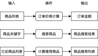
其中操作部分我们通常会直接编写程序代码实现,程序代码会查询数据库,使用某种算法处理数据等,这些工作可能很枯燥,一些程序员受不了了就会自称码农,因为日复一日编写这些逻辑就像种田一样艰苦和缺乏新意。你有没有想过如果有一套系统,可以只给出一些输入和输出的例子就能自动实现操作中的逻辑?如果有这么一套系统,在处理很多问题的时候就可以不需要考虑使用什么逻辑从输入转换到输出,我们只需提供一些例子这套系统就可以自动帮我们实现。
好消息是这样的系统是存在的,我们给出一些输入与输出的例子,让机器自动摸索出它们之间的规律并且建立一套转换它们的逻辑,就是所谓的机器学习。目前机器学习可以做到从图片识别出物体类别,从图片识别出文字,从文本识别出大概含义,也可以做到上图中的从已买商品列表计算出推荐商品列表,这些操作都不需要编写具体逻辑,只需要准备一定的例子让机器自己学习即可,如果成功摸索出规律,机器在遇到例子中没有的输入时也可以正确的计算出输出结果,如下图所示:

可惜的是机器学习不是万能的,我们不能指望机器可以学习到所有规律从而实现所有操作,机器学习的界限主要有:
- 做不到 100% 的精度,例如前述的根据商品列表计算订单价格要求非常准确,我们不能用机器学习来实现这个操作
- 需要一定的数据量,如果例子较少则无法成功学习到规律
- 无法实现复杂的判断,机器学习与人脑之间仍然有相当大的差距,一些复杂的操作无法使用机器学习代替
到这里我们应该对机器学习是什么有了一个大概的印象,如何根据输入与输出摸索出规律就是机器学习最主要的命题,接下来我们会更详细分析机器学习的流程与步骤。需要注意的是,不是所有场景都可以明确的给出输入与输出的例子,可以明确给出例子的学习称为有监督学习 (supervised learning),而只给出输入不给出输出例子的学习称为无监督学习 (unsupervised learning),无监督学习通常用于实现数据分类,虽然不给出输出但是会按一定的规律控制学习的过程,因为无监督学习应用范围不广,这个系列讲的基本上都是有监督学习。
2.2.机器学习的流程和步骤
先来了解一下机器学习的流程:

比如我这次要做的项目,识别是否佩戴口罩,输入一张图片转为灰度图读入计算机,设置相应的模型与参数,根据正确的数据集(即有监督学习)进行训练,计算损失根据损失调整参数,最后得到精度较高的训练模型以及参数。
而实现机器学习需要以下的步骤:
- 收集输入与输出的例子
- 建立模型
- 确定输入输出与模型可接收返回的数值之间如何转换
- 使用输入与输出的例子调整模型的参数
- 使用没有参与训练的输入与输出评价模型是否成功摸索出规律
2.2.1.收集输入与输出的例子
在开始机器学习之前我们需要先收集输入与输出的例子,收集到的例子又称数据集 (Dataset),收集工作一般是个苦力活,例如学习从图片判断物体类别需要收集一堆图片并手动对它们进行分类,学习从图片识别文字需要收集一堆图片并手动记录图片对应的文本,这样的工作通常称为打标签 (Labeling),标签 (Label) 就相当于这个数据对应的输出结果。有些时候我们也可以偷懒,例如实现验证码识别的时候我们可以反过来根据文本生成图片,然后把图片当作输入文本当作输出,再例如实现商品推荐的时候我们可以把用户购买过的商品分割成两部分,一部分作为已购买商品 (输入),另一部分作为推荐商品 (输出)。注意输入与输出可以有多个,例如视频网站可以根据用户的年龄,性别,所在地 (3 个输入) 来判断用户喜欢看的视频类型 (1 个输出),再例如自动驾驶系统可以根据视频输入,雷达输入与地图路线 (3 个输入) 计算汽车速度与方向盘角度 (2 个输出),后面会介绍如何处理多个输入与输出,包括数量可变的输入。
如果你只是想试试手而不是解决实际的业务问题,可以直接用别人收集好的数据集,以下是包含了各种公开数据集链接的 Github 仓库:
https://github.com/awesomedata/awesome-public-datasets
2.2.2.建立模型
用于让机器学习与实现操作的就是模型 (Model),模型可以分为两部分,第一部分是计算方法,这部分需要我们来决定并且不会在学习过程中改变;第二部分是参数,这部分会随着学习不断调整,最终实现我们想要的操作。模型的计算方法需要根据业务(输入与输出的类型)来决定,例如分类可以使用多层线性模型,图像识别可以使用 CNN 模型,趋势预测可以使用 RNN 模型,文本翻译可以使用 Transformer 模型,对象识别可以使用 R-CNN 模型等 (这些模型会在后续的章节详细介绍),通常我们可以直接用别人设计好的模型再加上一些细微调整(只会做这种工作的也叫调参狗,我们的第一个小目标),而一些复杂的业务需要自己设计模型,这是真正难的地方。你可能会想是否有一种模型可以适用于所有类型的业务,遗憾的是目前并没有,如果有那就是真正的人工智能了。
因为篇幅限制,现实使用的模型会在后面的文章中介绍,请参考本文末尾的预告。
2.2.3.确定输入输出与模型可接收返回的数值之间如何转换
在机器学习中,模型只会接受和返回数值 (通常使用多维数组,即矩阵),所以我们还需要决定输入输出与数值之间如何转换,例如输入是图片时,我们可以把每个像素的红绿蓝值与图片大小一起组成一个三维数组(红绿蓝 * 图片宽度 * 图片高度),再例如输入是数据库中的商品时,我们可以先根据总商品大小创建一个一维数组,然后用数组 1, 0, 0, ... 代表第一个商品,数组 0, 1, 0, ... 代表第二个商品,数组 0, 0, 1, ... 代表第三个商品,把数值转换到输出也一样,将对应关系反过来就行了。注意转换方式也是一个比较重要的部分,使用正确的转换方式可以让机器学习事半功倍,而使用错误的转换方式可能导致学习缓慢或学习失败。
为了提升学习速度,我们通常会一次性的给模型传入多组输入并让模型返回多组输出,传入的多组输入也叫批次 (Batch),例如准备了 10000 组输入与输出,每次给模型传入 50 组,那么批次大小就是 50,需要分 2000 个批次传入。分批次会让输入与输出的数组维度加一,例如一次性传 50 张宽 30 x 高 20 的图片时,需要把这些图片转换为一个 50 x 3 x 30 x 20 的四维数组,再例如传 50 个商品时,需要把这些商品转换为一个 50 x 商品数量的二维数组。你可能会有疑问为什么不能一次性把所有输入传给模型,如果输入输出数量过大(有的数据集会有上百万组数据),那么计算机不会有足够的内存处理它们;另一个原因是分批次传入可以防止过拟合 (Overfitting),但本篇不会详细介绍这点。惯例上,我们通常会选择 32 ~ 100 为批次大小。
此外,为了提升学习效果我们还可以选择把数值正规化 (Normalization),例如一个输入数值的取值范围在 0 ~ 10 的时候,我们可以把数值全部除以 10,用 0 代表最小的值,用 1 代表最大的值,这个手法可以改善模型的学习速度与提升最终的效果。因为理解需要一定的数学知识,本篇不会详细介绍为什么。
2.2.4.使用输入与输出的例子调整模型的参数
接下来我们就可以开始学习了,首先我们会给模型的参数 (非固定部分) 随机赋值,然后给模型传入预先准备好的输入,然后模型返回预测的输出,第一次因为参数是随机的,返回的预测输出与正确输出可能会差很远,例如传一张狗的图片给模型,模型可能会告诉你这是猪。接下来你需要纠正模型,把预测输出的数值与正确输出的数值通过某种方法得到它们的相差值 (也叫损失 - Loss),然后根据损失来调整模型的参数 (修改参数使得损失接近 0),让下一次模型的预测输出的数值更接近正确输出的数值。如果把事先准备的所有输入 (批次) 都传给了模型,并且根据模型的预测输出与正确输出调整了模型的参数,那么就可以说经过了一轮训练 (1 Epoch),通常我们需要经过好几轮训练才能达到理想的效果。

评价模型是否达到理想的效果通常会使用正确率 (Accuracy, 很多文章会缩写成 Acc),例如传入 100 个输入给模型,模型返回的 100 个预测输出中有 99 个与正确输出是一致的,那么正确率就是 99 %。如果模型足够强大,我们可以让模型针对参与训练的输入达到 100 % 的正确率,但这并不能说明模型训练成功,我们还需要使用没有参与训练的输入与输出来评价模型是否成功摸索出规律。如果模型能力不足,或者用了与业务不匹配的模型,那么模型会给出很低的正确率,并且经过再多训练都不会改善,这个时候我们就需要换一个模型了。模型通过训练达到很高的正确率又称收敛 (Converge),我们首先需要确定模型能收敛,再确定模型是否能成功摸索出规律。
2.2.5.使用没有参与训练的输入与输出评价模型是否成功摸索处规律(检验)
如果模型针对参与训练的输入达到了很高的正确率,那么就有两种情况,第一种情况是模型成功的摸索出规律了,第二种情况是模型只是把所有参与训练的输入与输出记住。第二种情况非常糟糕,就像我们把试卷的所有问题和答案记住了,但是没有理解为什么,遇到另一张没看过的试卷时就会得出很低的分数,这样的情况又称过拟合 (Overfitting)。
为了判断是否发生过拟合,我们通常会把事先准备好的输入与输出数据集打乱并分为三个集合,分别是训练集 (Training Set),验证集 (Validating Set) 与测试集 (Testing Set),举例来说我们可以把 70 % 的数据划给训练集,15 % 的数据划给验证集,剩余 15 % 的数据划给测试集。训练集中的输入与输出用于传给模型并且调整模型的参数;验证集中的输入与输出不会参与训练,用于在经过每一轮训练后判断模型在遇到未知的输入时可以得出的正确率,如果模型针对训练集可以得出 99 % 的正确率,但针对验证集只能得出 50 % 的正确率,那么就可以判断发生了过拟合;测试集用于在最终训练完成后判断模型是否过度偏向于训练集与验证集中的数据,如果针对测试集都可以得出比较高的正确率,那么就可以说这个模型训练成功了。
因为实际的业务场景中收集到的输入与输出会夹杂一些不完全正确的数据,如果不停的去训练模型,模型为了迎合这些不完全正确的数据会去破坏已经摸索出的规律,导致最终一定发生过拟合。为了防止这种情况我们可以使用提早停止 (Early Stopping) 的手法,在每一轮训练后都计算模型针对训练集与验证集的正确率,然后在验证集正确率最高的时候停止训练,例如:
- 第一轮训练后,训练集正确率 60 %,验证集正确率 58 %
- 第二轮训练后,训练集正确率 79 %,验证集正确率 72 %
- 第三轮训练后,训练集正确率 88 %,验证集正确率 86 %
- 第四轮训练后,训练集正确率 92 %,验证集正确率 85 %
- 第五轮训练后,训练集正确率 99 %,验证集正确率 78 %
我们可以看出应该在第三轮训练后停止训练,在实际操作中我们会记录每一轮训练的正确率与验证集正确率最高时模型的状态,如果验证集正确率经过一定训练次数都没有超过之前的最高值,那么就使用之前记录的模型状态作为结果并停止训练。在停止训练后,我们需要判断验证集正确率的最高值是否达到我们满意的水平,如果没有达到则代表模型不适合或者没有能力应付当前的业务,我们需要修改模型并重新开始训练。
如果验证集正确率的最高值达到我们满意的水平,那么就可以做最后一步了,即用模型判断测试集的正确率,因为测试集完全没有参与过之前的步骤,如果测试集的正确率也达到满意的水平,那么就可以说这个模型训练成功了。但如果测试集的正确率没有达到满意的水平,则代表模型对训练集与验证集有偏向,因为我们在验证集正确率不满意的时候会修改模型,修改后的模型会更偏向于验证集的数据,但这个偏向可能会不适合验证集以外的数据。训练集,验证集与测试集的意义可以总结如下:
- 训练集 (Training Set): 用于训练模型参数
- 验证集 (Validating Set): 用于判断模型是否支持处理没有训练过的输入,并手动调整模型的计算方法
- 测试集 (Testing Set): 用于最终判断模型是否支持处理完全没有参与训练与手动调整模型的输入
一个常见的人为错误是划分这三个集合的时候没有对数据进行打乱,例如有猫狗猪的图片各 1000 张,如果划分集合的时候这些图片是排序好的,那么训练集会只有猫和狗的图片,测试集会只有猪的图片,这样就很难确保训练出来的模型可以正确识别猪了。
从划分数据集到训练成功的流程可以总结如下:

注1: 让模型成功摸索出规律 (针对未知输入得出正确输出) 的工作一般称为泛化 (Generalization)。
注2: 防止过拟合还有另外一些手法,会在接下来的文章中介绍。
2.3.机器学习、深度学习和人工智能的区别
对初学者来说一个很常见的问题是,机器学习,深度学习与人工智能有什么区别?如果机器学习的模型非常复杂(经过多层次的计算),那么就可以说是深度学习,如果模型的效果非常好,在某个领域达到或者超过人类的水平,那就可以说是人工智能。但实际上它们都是 PPT 词汇,给投资人看的时候写人工智能比写机器学习要抢眼多了,就算不满足人工智能的水平很多公司都会宣传为人工智能。这个系列是给在 IT 食物链最底层的程序员看的,所以还是谦虚点叫机器学习吧。
2.4.一个最简单的例子
为了更好的理解前述的步骤,我准备了一个最简单的例子:
假设有以下的输入与输出,怎样才能自动找出从输入转换到输出的方法呢?

你很可能一眼就已经看出了它们的规律,别急,让我们使用机器学习来解决这个问题。
我们可以先假设输入乘以某个值再加上某个值等于输出,然后:
- 用 x 代表输入
- 用 y 代表输出
- 用 weight 代表输入乘以的值 (公式中缩写为 w)
- 用 bias 代表输出加上的值 (公式中缩写为 b)
用数学公式可以表达如下:
![]()
这个公式就是模型中的计算方法部分,而 weight 和 bias 则是这个模型的参数,我们把部分输入与输出代入 x 和 y:
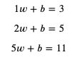
接下来要做的就是找出可以满足这些等式的 weight 和 bias。
我们首先随便给 weight 和 bias 分配值,例如给 weight 分配 1,给 bias 分配 0,然后试试计算结果:
![]()
这个计算结果 2 就是预测输出,而预测输出和正确输出之间的差距就是损失。
如果用 predicted (缩写 p) 代表预测输出,用 loss (缩写 l) 代表损失,可以得出以下公式:

如果 loss 等于 0,那么预测输出 predicted 就会等于正确输出 y,我们的目标是尽量的让 loss 接近 0。
想想如果 weight 增加 1 时 loss 会增加多少,而 bias 增加 1 时 loss 会增加多少:
- weight 增加 1 时,loss 会增加 x
- bias 增加 1 时,loss 会增加 1
可以看出 weight 和 bias 与 loss 是正相关的,并且 weight 和 bias 对 loss 的贡献是 x 比 1,在前面的例子中,loss 等于 predicted - y 等于 2 - 5 等于 -3,我们需要增加 weight 和 bias 的值来让 loss 更接近 0。增加 weight 和 bias 时的比例应该与贡献比例一致,试着给 weight 加上 x,bias 加上 1,调整以后 weight 等于 3,bias 等于 1,计算结果如下:
![]()
这下 loss 等于 7 - 5 等于 2 了,我们需要减少 weight 和 bias 来让 loss 更接近 0,如果和之前一样 weight 减去 x,bias 减去 1,那么 weight 和 bias 就会变回之前的值,不管调整多少次都无法减少 loss,噢。解决这个问题可以控制每次 weight 和 bias 的修改量,例如每次只修改 0.01 倍 (这个倍数又称学习比率 - Learning Rate - 简称 LR),总结规则如下:
如果 loss 小于 0:
- weight 增加 x 乘以 0.01
- bias 增加 0.01
如果 loss 大于 0:
- weight 减少 x 乘以 0.01
- bias 减少 0.01
模拟一下修改的过程:
第一轮:
x = 2, y = 5, weight = 1, bias = 0
predicted = 2 * 1 + 0 = 2
loss = 2 - 5 = -3
weight += 2 * 0.1
bias += 0.1第二轮:
x = 2, y = 5, weight = 1.02, bias = 0.01
predicted = 2 * 1.02 + 0.01 = 2.05
loss = 2.05 - 5 = -2.95
weight += 2 * 0.1
bias += 0.1第三轮:
x = 2, y = 5, weight = 1.04, bias = 0.02
predicted = 2 * 1.04 + 0.02 = 2.1
loss = 2.1 - 5 = -2.9
weight += 2 * 0.1
bias += 0.1
可以看到 loss 越来越接近 0,继续修改下去 weight 会等于 2.2,bias 会等于 0.6,满足 x 等于 2,y 等于 5 的情况,但满足不了数据集中的其他数据。我们可以编写一个程序遍历数据集中的数据来进行同样的修改,来看看能不能找到满足数据集中所有数据的 weight 和 bias:
# 定义参数
weight = 1
bias = 0

# 定义学习比率
learning_rate = 0.01

# 准备训练集,验证集和测试集
traning_set = [(2, 5), (5, 11), (6, 13), (7, 15), (8, 17)]
validating_set = [(12, 25), (1, 3)]
testing_set = [(9, 19), (13, 27)]

for epoch in range(1, 10000):
    print(f"epoch: {epoch}")

    # 根据训练集训练并修改参数
    for x, y in traning_set:
        # 计算预测值
        predicted = x * weight + bias
        # 计算损失
        loss = predicted - y
        # 打印除错信息
        print(f"traning x: {x}, y: {y}, predicted: {predicted}, loss: {loss}, weight: {weight}, bias: {bias}")
        # 判断需要如何修改 weight 和 bias 才能减少 loss
        if loss < 0:
            # 需要增加 weight 和 bias 来让 predicted 更大
            weight += x * learning_rate
            bias += 1 * learning_rate
        else:
            # 需要减少 weight 和 bias 来让 predicted 更小
            weight -= x * learning_rate
            bias -= 1 * learning_rate

    # 检查验证集
    validating_accuracy = 0
    for x, y in validating_set:
        predicted = x * weight + bias
        validating_accuracy += 1 - abs(y - predicted) / y
        print(f"validating x: {x}, y: {y}, predicted: {predicted}")
    validating_accuracy /= len(validating_set)

    # 如果验证集正确率大于 99 %,则停止训练
    print(f"validating accuracy: {validating_accuracy}")
    if validating_accuracy > 0.99:
        break

# 检查测试集
testing_accuracy = 0
for x, y in testing_set:
    predicted = x * weight + bias
    testing_accuracy += 1 - abs(y - predicted) / y
    print(f"testing x: {x}, y: {y}, predicted: {predicted}")
testing_accuracy /= len(testing_set)
print(f"testing accuracy: {testing_accuracy}")
输出结果如下:
D:\anaconda\envs\pythonProject2\python.exe D:/Pycharm_Projects/pythonProject2/easiest_example1.py
epoch: 1
traning x: 2, y: 5, predicted: 2, loss: -3, weight: 1, bias: 0
traning x: 5, y: 11, predicted: 5.109999999999999, loss: -5.890000000000001, weight: 1.02, bias: 0.01
traning x: 6, y: 13, predicted: 6.4399999999999995, loss: -6.5600000000000005, weight: 1.07, bias: 0.02
traning x: 7, y: 15, predicted: 7.940000000000001, loss: -7.059999999999999, weight: 1.1300000000000001, bias: 0.03
traning x: 8, y: 17, predicted: 9.64, loss: -7.359999999999999, weight: 1.2000000000000002, bias: 0.04
validating x: 12, y: 25, predicted: 15.410000000000004
validating x: 1, y: 3, predicted: 1.3300000000000003
validating accuracy: 0.5298666666666668
epoch: 2
traning x: 2, y: 5, predicted: 2.6100000000000003, loss: -2.3899999999999997, weight: 1.2800000000000002, bias: 0.05
traning x: 5, y: 11, predicted: 6.560000000000001, loss: -4.439999999999999, weight: 1.3000000000000003, bias: 0.060000000000000005
traning x: 6, y: 13, predicted: 8.170000000000002, loss: -4.829999999999998, weight: 1.3500000000000003, bias: 0.07
traning x: 7, y: 15, predicted: 9.950000000000003, loss: -5.049999999999997, weight: 1.4100000000000004, bias: 0.08
traning x: 8, y: 17, predicted: 11.930000000000003, loss: -5.069999999999997, weight: 1.4800000000000004, bias: 0.09
validating x: 12, y: 25, predicted: 18.820000000000007
validating x: 1, y: 3, predicted: 1.6600000000000006
validating accuracy: 0.6530666666666669省略中间
epoch: 90
traning x: 2, y: 5, predicted: 4.949999999999935, loss: -0.05000000000006466, weight: 1.9799999999999676, bias: 0.9900000000000007
traning x: 5, y: 11, predicted: 10.999999999999838, loss: -1.616484723854228e-13, weight: 1.9999999999999676, bias: 1.0000000000000007
traning x: 6, y: 13, predicted: 13.309999999999807, loss: 0.3099999999998069, weight: 2.0499999999999674, bias: 1.0100000000000007
traning x: 7, y: 15, predicted: 14.929999999999772, loss: -0.07000000000022766, weight: 1.9899999999999674, bias: 1.0000000000000007
traning x: 8, y: 17, predicted: 17.48999999999974, loss: 0.4899999999997391, weight: 2.059999999999967, bias: 1.0100000000000007
validating x: 12, y: 25, predicted: 24.759999999999607
validating x: 1, y: 3, predicted: 2.9799999999999676
validating accuracy: 0.9918666666666534
testing x: 9, y: 19, predicted: 18.819999999999705
testing x: 13, y: 27, predicted: 26.739999999999572
testing accuracy: 0.9904483430799063Process finished with exit code 0
最终 weight 等于 2.05,bias 等于 1.01,它针对没有训练过的检查集和测试集可以达到 99 % 的正确率 (预测输出 99 % 接近正确输出),如果 99 % 的正确率可以接受,那么就可以说这次训练成功了。
如果你想看 weight 和 bias 的变化,可以记录它们的值并且使用 matplotlib 来显示图表。
安装 matplotlib 的命令:
pip3 install matplotlib
修改后的代码:
# 定义参数
weight = 1
bias = 0

# 定义学习比率
learning_rate = 0.01

# 准备训练集,验证集和测试集
traning_set = [(2, 5), (5, 11), (6, 13), (7, 15), (8, 17)]
validating_set = [(12, 25), (1, 3)]
testing_set = [(9, 19), (13, 27)]

# 记录 weight 与 bias 的历史值
weight_history = [weight]
bias_history = [bias]

for epoch in range(1, 10000):
    print(f"epoch: {epoch}")

    # 根据训练集训练并修改参数
    for x, y in traning_set:
        # 计算预测值
        predicted = x * weight + bias
        # 计算损失
        loss = predicted - y
        # 打印除错信息
        print(f"traning x: {x}, y: {y}, predicted: {predicted}, loss: {loss}, weight: {weight}, bias: {bias}")
        # 判断需要如何修改 weight 和 bias 才能减少 loss
        if loss < 0:
            # 需要增加 weight 和 bias 来让 predicted 更大
            weight += x * learning_rate
            bias += 1 * learning_rate
        else:
            # 需要减少 weight 和 bias 来让 predicted 更小
            weight -= x * learning_rate
            bias -= 1 * learning_rate
        weight_history.append(weight)
        bias_history.append(bias)

    # 检查验证集
    validating_accuracy = 0
    for x, y in validating_set:
        predicted = x * weight + bias
        validating_accuracy += 1 - abs(y - predicted) / y
        print(f"validating x: {x}, y: {y}, predicted: {predicted}")
    validating_accuracy /= len(validating_set)

    # 如果验证集正确率大于 99 %,则停止训练
    print(f"validating accuracy: {validating_accuracy}")
    if validating_accuracy > 0.99:
        break

# 检查测试集
testing_accuracy = 0
for x, y in testing_set:
    predicted = x * weight + bias
    testing_accuracy += 1 - abs(y - predicted) / y
    print(f"testing x: {x}, y: {y}, predicted: {predicted}")
testing_accuracy /= len(testing_set)
print(f"testing accuracy: {testing_accuracy}")

# 显示 weight 与 bias 的变化
from matplotlib import pyplot
pyplot.plot(weight_history, label="weight")
pyplot.plot(bias_history, label="bias")
pyplot.legend()
pyplot.show()
输出的图表,可以看到 weight 接近 2 以后一直上下浮动,而 bias 逐渐接近 1:

等等,你是不是觉得这个例子很蠢?这个例子的确很蠢,如果我们用其他方法 (例如联立方程式) 可以马上计算出 weight 应该等于 2,bias 应该等于 1,这时预测输出 100 % 等于正确输出。但这个例子代表了机器学习最基础的原理 - 计算各个参数对损失的贡献比例然后修改参数让损失接近 0,如果模型的计算方法非常复杂,将没有方法立刻计算出可以让损失等于 0 的参数值,只能慢慢的调整参数去试。
好了,那为什么上面的例子不能调整 weight 到 2,bias 到 1 呢?主要有两个原因,第一是学习比率为 0.01,如果出现 loss 很接近但小于 0,weight 和 bias 增加以后 loss 大于 0,然后减少 weight 和 bias 又让 loss 变回原来的值,那么接下来无论学习多少次 loss 都不会等于 0,而是在小于 0 的某个值和大于 0 的某个值之间摇摆;第二是我们在正确率达到 99 % 的时候就中断了训练。你可以试试减少学习比率和增加中断训练需要的正确率,试试 weight 和 bias 会不会更接近 2 和 1。
此外在这个例子中,因为所有数据都是完美的,没有杂质在里面,并且模型非常的简单,所以不会出现过拟合 (Overfitting) 问题,也不需要使用提早停止 (Early Stopping) 的手法来防止过拟合。
2.5.机器学习
很多机器学习的文章喜欢用抛物线和一个球来形容机器学习训练的过程:

把球看作参数,抛物线看作 loss 的值,如果球在左半部分 loss 小于 0,如果球在右半部分 loss 大于 0,如果球落在最低点那么 loss 等于 0,机器学习的过程就是调整这个球的位置。球所在的位置的梯度 (Gradient) 决定了球的移动方向和每次的移动距离(移动速度),球在左半边的时候会向右移,球在右半边的时候会向左移,而梯度越大每次的移动距离就越长,如果每次的移动距离很长,球可能会一直左右摇摆而无法落在最低点,这个时候我们就需要使用学习比率 (Learning Rate) 来控制每次移动的距离,让每次移动的距离等于 梯度 * 学习比率。
在前述的例子中,参数 weight 的梯度是 x,而参数 bias 的梯度是 1,这实际上就是它们的导函数 (Derivative Function):

如果你还记得高中学过的微积分,那么立刻就能看明白,但我问过但很多程序员都说已经忘光了还给数学老师了,所以我在这里再简单解释一下微分的概念,还记得的就当复习叭。
所谓微分就是求某个函数的导函数,而导函数就是求某一个点上值的变化与结果的变化的关联 (梯度)。以前面的例子为例,weight 如果增加 1,那么 loss 就会增加 x,weight 如果增加 2,那么 loss 就会增加 2x,所以 weight 的导函数可以用 x 来表示;而 bias 如果增加 1,那么 loss 就会增加 1,bias 如果增加 2,那么 loss 就会增加 2,所以 bias 的导函数可以用 1 来表示。
求导函数的通用公式如下:

求 weight 和 bias 的导函数 (weight 和 bias 的变化与 loss 的变化的关联) 的过程如下:
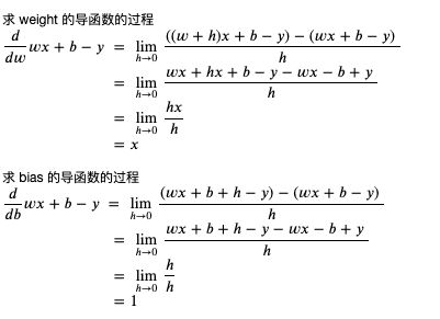
你可能会有疑问为什么要求 h 无限接近于 0,这是因为导函数求的是某个点上变化的关联,而这个关联可能会根据点的位置而不同,在上述例子中 weight 和 bias 不管在哪里,它们和 loss 的关联都是相同的,不会依赖于 weight 和 bias 的值。我们可以看一个根据位置不同关联发生变化的例子,例如 x 的平方:
当 x 等于 3 时,x 的平方等于 9
当 x 等于 5 时,x 当平方等于 25求 x 的变化与 x 的平方的变化的关联
当 x 等于 3 + 1 时,x 的平方等于 16,与原值相差 7
当 x 等于 5 + 1 时,x 当平方等于 36,与原值相差 11可以看到当 x 增加 1 时,x 的平方增加多少不是固定的,会依赖于 x 的值
求 x 的平方的导函数的过程如下:

我们可以粗略检查一下这个导函数是否正确 (以下的代码运行在 python 的 REPL 中):
>>> ((3 + 1) ** 2 - 3 ** 2) / 1
7.0
>>> ((3 + 0.1) ** 2 - 3 ** 2) / 0.1
6.100000000000012
>>> ((3 + 0.01) ** 2 - 3 ** 2) / 0.01
6.009999999999849
>>> ((3 + 0.001) ** 2 - 3 ** 2) / 0.001
6.000999999999479
>>> ((5 + 1) ** 2 - 5 ** 2) / 1
11.0
>>> ((5 + 0.1) ** 2 - 5 ** 2) / 0.1
10.09999999999998
>>> ((5 + 0.01) ** 2 - 5 ** 2) / 0.01
10.009999999999764
>>> ((5 + 0.001) ** 2 - 5 ** 2) / 0.001
10.001000000002591
可以看到变化的值越接近 0,变化值与结果的关联越接近 2x。
现在我们了解微分了,那积分是什么呢?积分分为不定积分和定积分,不定积分就是反过来从导函数求原始函数,定积分就是从导函数和参数的变化范围求结果的变化范围:

好了,复习就到此为止,我们来总结一下机器学习是怎么利用微分来调整参数的:
- 假设一个可以从输入计算输出的公式
- 定好计算损失的方法,并把公式变形为计算损失的公式
- 利用微分来计算公式的各个参数对损失的贡献比例 (也就是偏导)
- 随机分配参数的值
- 用预先收集好的输入计算预测输出,然后用预测输出和正确输出计算损失
- 根据各个参数对损失的贡献比例调整参数,使得损失接近 0
- 损失非常接近 0 时,代表公式计算的预测输出非常接近正确输出,如果达到可接受的范围就可以停止训练
这种调整参数方式称为梯度下降法 (Gradient Descent),因为参数的值是随机分配的,通常又称为随机梯度下降法 (Stochastic Gradient Descent, 简称 SGD)。
2.6.让参数调整量依赖于损失的
我们再来回头看看前面的例子,会发现调整参数的时候,调整量只会依赖输入与学习比率,不会依赖损失的大小,如果我们想在损失比较大的时候调整多一点,损失比较小的时候调整少一点,应该怎么办呢?
我们可以改变损失的计算方法,把预测输出和正确输出相差的值的平方作为损失,这里我引入一个新的临时变量 diff (缩写 d) 来表示预测输出和正确输出相差的值:

这个时候应该如何计算 weight 和 bias 的导函数呢?

我们可以使用连锁律 (Chain Rule),简单的来说就是如果 x 的变化影响了 y 的变化,y 的变化影响了 z 的变化,那么 x 的变化 与 z 的变化之间的关系可以用前面两个变化的关系组合计算出来 (注意下图中的公式用的是 Lagrange's notation,只是记法不一样):
![]()
使用连锁律计算 weight 和 bias 的导函数的过程如下 (如果你有兴趣和时间可以试试不用连锁律计算,看看结果是否一样):

可以看到修改 loss 的计算方式后,weight 和 bias 对 loss 的贡献比例是 2 * diff * x 比 2 * diff,会依赖于预测输出与正确输出相差的值,现在我们修改一下上面例子的代码,看看是否仍然可以训练成功:
# 定义参数
weight = 1
bias = 0

# 定义学习比率
learning_rate = 0.01

# 准备训练集,验证集和测试集
traning_set = [(2, 5), (5, 11), (6, 13), (7, 15), (8, 17)]
validating_set = [(12, 25), (1, 3)]
testing_set = [(9, 19), (13, 27)]

# 记录 weight 与 bias 的历史值
weight_history = [weight]
bias_history = [bias]

for epoch in range(1, 10000):
    print(f"epoch: {epoch}")

    # 根据训练集训练并修改参数
    for x, y in traning_set:
        # 计算预测值
        predicted = x * weight + bias
        # 计算损失
        diff = predicted - y
        loss = diff ** 2
        # 打印除错信息
        print(f"traning x: {x}, y: {y}, predicted: {predicted}, loss: {loss}, weight: {weight}, bias: {bias}")
        # 计算导函数值
        derivative_weight = 2 * diff * x
        derivative_bias = 2 * diff
        # 修改 weight 和 bias 以减少 loss
        # diff 为正时代表预测输出 > 正确输出,会减少 weight 和 bias
        # diff 为负时代表预测输出 < 正确输出,会增加 weight 和 bias
        weight -= derivative_weight * learning_rate
        bias -= derivative_bias * learning_rate
        # 记录 weight 和 bias 的历史值
        weight_history.append(weight)
        bias_history.append(bias)

    # 检查验证集
    validating_accuracy = 0
    for x, y in validating_set:
        predicted = x * weight + bias
        validating_accuracy += 1 - abs(y - predicted) / y
        print(f"validating x: {x}, y: {y}, predicted: {predicted}")
    validating_accuracy /= len(validating_set)

    # 如果验证集正确率大于 99 %,则停止训练
    print(f"validating accuracy: {validating_accuracy}")
    if validating_accuracy > 0.99:
        break

# 检查测试集
testing_accuracy = 0
for x, y in testing_set:
    predicted = x * weight + bias
    testing_accuracy += 1 - abs(y - predicted) / y
    print(f"testing x: {x}, y: {y}, predicted: {predicted}")
testing_accuracy /= len(testing_set)
print(f"testing accuracy: {testing_accuracy}")

# 显示 weight 与 bias 的变化
from matplotlib import pyplot
pyplot.plot(weight_history, label="weight")
pyplot.plot(bias_history, label="bias")
pyplot.legend()
pyplot.show()
epoch: 1
traning x: 2, y: 5, predicted: 2, loss: 9, weight: 1, bias: 0
traning x: 5, y: 11, predicted: 5.66, loss: 28.5156, weight: 1.12, bias: 0.06
traning x: 6, y: 13, predicted: 10.090800000000002, loss: 8.463444639999992, weight: 1.6540000000000001, bias: 0.1668
traning x: 7, y: 15, predicted: 14.246711999999999, loss: 0.567442810944002, weight: 2.003104, bias: 0.22498399999999996
traning x: 8, y: 17, predicted: 17.108564320000003, loss: 0.011786211577063013, weight: 2.10856432, bias: 0.24004976
validating x: 12, y: 25, predicted: 25.332206819199993
validating x: 1, y: 3, predicted: 2.3290725023999994
validating accuracy: 0.8815346140160001
epoch: 2
traning x: 2, y: 5, predicted: 4.420266531199999, loss: 0.3360908948468813, weight: 2.0911940287999995, bias: 0.23787847359999995
traning x: 5, y: 11, predicted: 10.821389980735997, loss: 0.03190153898148744, weight: 2.1143833675519996, bias: 0.24947314297599996
traning x: 6, y: 13, predicted: 13.046511560231679, loss: 0.0021633252351850635, weight: 2.1322443694784, bias: 0.25304534336128004
traning x: 7, y: 15, predicted: 15.138755987910837, loss: 0.019253224181112433, weight: 2.1266629822505987, bias: 0.25211511215664645
traning x: 8, y: 17, predicted: 17.10723714394308, loss: 0.011499805041069082, weight: 2.1072371439430815, bias: 0.2493399923984297
validating x: 12, y: 25, predicted: 25.32814566046583
validating x: 1, y: 3, predicted: 2.3372744504317566
validating accuracy: 0.8829828285293095
epoch: 3
traning x: 2, y: 5, predicted: 4.427353651343945, loss: 0.327923840629112, weight: 2.0900792009121885, bias: 0.24719524951956806
traning x: 5, y: 11, predicted: 10.823573450784844, loss: 0.03112632726796794, weight: 2.112985054858431, bias: 0.2586481764926892
traning x: 6, y: 13, predicted: 13.045942966156671, loss: 0.0021107561392730407, weight: 2.1306277097799464, bias: 0.2621767074769923
traning x: 7, y: 15, predicted: 15.13705972504188, loss: 0.01878536822855566, weight: 2.125114553841146, bias: 0.2612578481538589
traning x: 8, y: 17, predicted: 17.105926192335282, loss: 0.011220358222651178, weight: 2.1059261923352826, bias: 0.2585166536530213
validating x: 12, y: 25, predicted: 25.324134148545966
validating x: 1, y: 3, predicted: 2.3453761313679533
validating accuracy: 0.8844133389237396省略途中的输出
epoch: 202
traning x: 2, y: 5, predicted: 4.950471765167672, loss: 0.002453046045606255, weight: 2.0077909582882314, bias: 0.9348898485912089
traning x: 5, y: 11, predicted: 10.984740851695477, loss: 0.00023284160697942092, weight: 2.0097720876815246, bias: 0.9358804132878555
traning x: 6, y: 13, predicted: 13.003973611325808, loss: 1.578958696858945e-05, weight: 2.011298002511977, bias: 0.936185596253946
traning x: 7, y: 15, predicted: 15.011854308097591, loss: 0.00014052462047262272, weight: 2.01082116915288, bias: 0.9361061240274299
traning x: 8, y: 17, predicted: 17.009161566019216, loss: 8.393429192445584e-05, weight: 2.0091615660192175, bias: 0.935869037865478
validating x: 12, y: 25, predicted: 25.02803439201881
validating x: 1, y: 3, predicted: 2.9433815220012365
validating accuracy: 0.9900028991598299
testing x: 9, y: 19, predicted: 19.00494724565038
testing x: 13, y: 27, predicted: 27.03573010747495
testing accuracy: 0.9992081406680464
weight 与 bias 的变化如下:

你可能会发现训练速度比前面的例子慢很多,这是因为这个例子实在太简单了,所以无法显示出让参数调整量依赖损失的优势,在复杂的场景下它可以让训练速度更快并且让预测输出更接近正确输出。此外,还有另外一些计算损失的方法,例如 Cross Entropy 等,它们将在后面的文章中提到。
最后补充一个知识点,通过输入计算预测输出的过程在机器学习中称作 Forward,而通过损失调整参数的过程则称作 Backward,如果参数经过多层计算,那么可以把调整多层参数的过程称为反向传播 (Backpropagation),多层计算的模型将在后面的文章中提到。
三.pytorch与矩阵计算入门
3.1.Pytorch简介
pytorch 是目前世界上最流行的两个机器学习框架的其中之一,与 tensoflow 并峙双雄。它提供了很多方便的功能,例如根据损失自动微分计算应该怎样调整参数,提供了一系列的数学函数封装,还提供了一系列现成的模型,以及把模型组合起来进行训练的框架。pytorch 的前身是 torch,基于 lua,而 pytorch 基于 python,虽然它基于 python 但底层完全由 c++ 编写,支持自动并列化计算和使用 GPU 加速运算,所以它的性能非常好。
传统的机器学习有的会像前一节的例子中全部手写,或者利用 numpy 类库减少一部分工作量,也有人会利用 scikit-learn (基于 numpy) 类库封装好的各种经典算法。pytorch 与 tensorflow 和传统机器学习不一样的是,它们把重点放在了组建类似人脑的神经元网络 (Neural Network),所以能实现传统机器学习无法做到的非常复杂的判断,例如判断图片中的物体类型,自动驾驶等。不过,它们组建的神经元网络工作方式是不是真的和人脑类似仍然有很多争议,目前已经有人开始着手组建原理上更接近人脑的 GNN (Graph Neural Network) 网络,但仍未实用化,所以我们这个系列还是会着重讲解当前已经实用化并广泛应用在各个行业的网络模型。
3.2.学Pytorch好还是Tensorflow好?
对初学者来说一个很常见的问题是,学 pytorch 还是学 tensorflow 好?按目前的统计数据来说,公司更多使用 tensorflow,而研究人员更多使用 pytorch,pytorch 的增长速度非常快,有超越 tensorflow 的趋势。我的意见是学哪个都无所谓,如果你熟悉 pytorch,学 tensorflow 也就一两天的事情,反过来也一样,并且 pytorch 和 tensorflow 的项目可以互相移植,选一个觉得好学的就可以了。因为我觉得 pytorch 更好学 (封装非常直观,使用 Dynamic Graph 使得调试非常容易),所以这个系列会基于 pytorch 来讲。
3.2.1.Dynamic Graph 与 Static Graph
机器学习框架按运算的流程是否需要预先固定可以分为 Dynamic Graph 和 Static Graph,Dynamic Graph 不需要预先固定运算流程,而 Static Graph 需要。举例来说,对同一个公式 wx + b = y,Dynamic Graph 型的框架可以把 wx,+b 分开写并且逐步计算,计算的过程中随时都可以用 print 等指令输出途中的结果,或者把途中的结果发送到其他地方记录起来;而 Static Graph 型的框架必须预先定好整个计算流程,你只能传入 w, x, b 给计算器,然后让计算器输出 y,中途计算的结果只能使用专门的调试器来查看。
一般的来说 Static Graph 性能会比 Dynamic Graph 好,Tensorflow (老版本) 使用的是 Static Graph,而 pytorch 使用的是 Dynamic Graph,但两者实际性能相差很小,因为消耗资源的大部分都是矩阵运算,使用批次训练可以很大程度减少它们的差距。顺带一提,Tensorflow 1.7 开始支持了 Dynamic Graph,并且在 2.0 默认开启,但大部分人在使用 Tensorflow 的时候还是会用 Static Graph。
我本次使用的Faster-RCNN要使用Dynamic Graph以便中途输出结果便于写技术文档。
# Dynamic Graph 的印象,运算的每一步都可以插入自定义代码
def forward(w, x, b):
    wx = w * x
    print(wx)
    y = wx + b
    print(y)
    return y
forward(w, x, b)

# Static Graph 的印象,需要预先编译整个计算流程
forward = compile("wx+b")
forward(w, x, b)
3.3.安装Pytorch
pip3 install pytorch
之后在 python 代码中使用 import torch 即可引用 pytorch 类库。
3.4.Pytorch
接下来我们熟悉一下 pytorch 里面最基本的操作,pytorch 会用 torch.Tensor 类型来统一表现数值,向量 (一维数组) 或矩阵 (多维数组),模型的参数也会使用这个类型。(tensorflow 会根据用途分为好几个类型,这点 pytorch 更简洁明了)
torch.Tensor 类型可以使用 torch.tensor 函数构建,以下是一些简单的例子(运行在 python 的 REPL 中):
# 引用 pytorch
>>> import torch

# 创建一个整数 tensor
>>> torch.tensor(1)
tensor(1)

# 创建一个小数 tensor
>>> torch.tensor(1.0)
tensor(1.)

# 单值 tensor 中的值可以用 item 函数取出
>>> torch.tensor(1.0).item()
1.0

# 使用一维数组创建一个向量 tensor
>>> torch.tensor([1.0, 2.0, 3.0])
tensor([1., 2., 3.])

# 使用二维数组创建一个矩阵 tensor
>>> torch.tensor([[1.0, 2.0, 3.0], [-1.0, -2.0, -3.0]])
tensor([[ 1.,  2.,  3.],
        [-1., -2., -3.]])
tensor 对象的数值类型可以看它的 dtype 成员:
>>> torch.tensor(1).dtype
torch.int64
>>> torch.tensor(1.0).dtype
torch.float32
>>> torch.tensor([1.0, 2.0, 3.0]).dtype
torch.float32
>>> torch.tensor([[1.0, 2.0, 3.0], [-1.0, -2.0, -3.0]]).dtype
torch.float32
pytorch 支持整数类型 torch.uint8, torch.int8, torch.int16, torch.int32, torch.int64 ,浮点数类型 torch.float16, torch.float32, torch.float64,还有布尔值类型 torch.bool。类型后的数字代表它的位数 (bit 数),而 uint8 前面的 u 代表它是无符号数 (unsigned)。实际绝大部分场景都只会使用 torch.float32,虽然精度没有 torch.float64 高但它占用内存小并且运算速度快。注意一个 tensor 对象里面只能保存一种类型的数值,不能混合存放。
创建 tensor 对象时可以通过 dtype 参数强制指定类型:
>>> torch.tensor(1, dtype=torch.int32)
tensor(1, dtype=torch.int32)
>>> torch.tensor([1.1, 2.9, 3.5], dtype=torch.int32)
tensor([1, 2, 3], dtype=torch.int32)

>>> torch.tensor(1, dtype=torch.int64)
tensor(1)

>>> torch.tensor(1, dtype=torch.float32)
tensor(1.)

>>> torch.tensor(1, dtype=torch.float64)
tensor(1., dtype=torch.float64)
>>> torch.tensor([1, 2, 3], dtype=torch.float64)
tensor([1., 2., 3.], dtype=torch.float64)

>>> torch.tensor([1, 2, 0], dtype=torch.bool)
tensor([ True,  True, False])
tensor 对象的形状可以看它的 shape 成员:
# 整数 tensor 的 shape 为空
>>> torch.tensor(1).shape
torch.Size([])
>>> torch.tensor(1.0).shape
torch.Size([])

# 数组 tensor 的 shape 只有一个值,代表数组的长度
>>> torch.tensor([1.0]).shape
torch.Size([1])
>>> torch.tensor([1.0, 2.0, 3.0]).shape
torch.Size([3])

# 矩阵 tensor 的 shape 根据它的维度而定,每个值代表各个维度的大小,这个例子代表矩阵有 2 行 3 列
>>> torch.tensor([[1.0, 2.0, 3.0], [-1.0, -2.0, -3.0]]).shape
torch.Size([2, 3])
tensor 对象与数值,tensor 对象与 tensor 对象之间可以进行运算:
>>> torch.tensor(1.0) * 2
tensor(2.)
>>> torch.tensor(1.0) * torch.tensor(2.0)
tensor(2.)
>>> torch.tensor(3.0) * torch.tensor(2.0)
tensor(6.)
向量和矩阵还可以批量进行运算(内部会并列化运算):
# 向量和数值之间的运算
>>> torch.tensor([1.0, 2.0, 3.0])
tensor([1., 2., 3.])
>>> torch.tensor([1.0, 2.0, 3.0]) * 3
tensor([3., 6., 9.])
>>> torch.tensor([1.0, 2.0, 3.0]) * 3 - 1
tensor([2., 5., 8.])

# 矩阵和单值 tensor 对象之间的运算
>>> torch.tensor([[1.0, 2.0, 3.0], [-1.0, -2.0, -3.0]])
tensor([[ 1.,  2.,  3.],
        [-1., -2., -3.]])
>>> torch.tensor([[1.0, 2.0, 3.0], [-1.0, -2.0, -3.0]]) / torch.tensor(2)
tensor([[ 0.5000,  1.0000,  1.5000],
        [-0.5000, -1.0000, -1.5000]])

# 矩阵和与矩阵最后一个维度相同长度向量之间的运算
>>> torch.tensor([[1.0, 2.0, 3.0], [-1.0, -2.0, -3.0]]) * torch.tensor([1.0, 1.5, 2.0])
tensor([[ 1.,  3.,  6.],
        [-1., -3., -6.]])
tensor 对象之间的运算一般都会生成一个新的 tensor 对象,如果你想避免生成新对象 (提高性能),可以使用 _ 结尾的函数,它们会修改原有的对象:
# 生成新对象,原有对象不变,add 和 + 意义相同
>>> a = torch.tensor([1,2,3])
>>> b = torch.tensor([7,8,9])
>>> a.add(b)
tensor([ 8, 10, 12])
>>> a
tensor([1, 2, 3])

# 在原有对象上执行操作,避免生成新对象
>>> a.add_(b)
tensor([ 8, 10, 12])
>>> a
tensor([ 8, 10, 12])
pytorch 还提供了一系列方便的函数求最大值,最小值,平均值,标准差等:
>>> torch.tensor([1.0, 2.0, 3.0])
tensor([1., 2., 3.])
>>> torch.tensor([1.0, 2.0, 3.0]).min()
tensor(1.)
>>> torch.tensor([1.0, 2.0, 3.0]).max()
tensor(3.)
>>> torch.tensor([1.0, 2.0, 3.0]).mean()
tensor(2.)
>>> torch.tensor([1.0, 2.0, 3.0]).std()
tensor(1.)
pytorch 还支持比较 tensor 对象来生成布尔值类型的 tensor:
# tensor 对象与数值比较
>>> torch.tensor([1.0, 2.0, 3.0]) > 1.0
tensor([False,  True,  True])
>>> torch.tensor([1.0, 2.0, 3.0]) <= 2.0
tensor([ True,  True, False])

# tensor 对象与 tensor 对象比较
>>> torch.tensor([1.0, 2.0, 3.0]) > torch.tensor([1.1, 1.9, 3.0])
tensor([False,  True, False])
>>> torch.tensor([1.0, 2.0, 3.0]) <= torch.tensor([1.1, 1.9, 3.0])
tensor([ True, False,  True])
pytorch 还支持生成指定形状的 tensor 对象:
# 生成 2 行 3 列的矩阵 tensor,值全部为 0
>>> torch.zeros(2, 3)
tensor([[0., 0., 0.],
        [0., 0., 0.]])

# 生成 3 行 2 列的矩阵 tensor,值全部为 1
torch.ones(3, 2)
>>> torch.ones(3, 2)
tensor([[1., 1.],
        [1., 1.],
        [1., 1.]])

# 生成 3 行 2 列的矩阵 tensor,值全部为 100
>>> torch.full((3, 2), 100)
tensor([[100., 100.],
        [100., 100.],
        [100., 100.]])

# 生成 3 行 3 列的矩阵 tensor,值为范围 [0, 1) 的随机浮点数
>>> torch.rand(3, 3)
tensor([[0.4012, 0.2412, 0.1532],
        [0.1178, 0.2319, 0.4056],
        [0.7879, 0.8318, 0.7452]])

# 生成 3 行 3 列的矩阵 tensor,值为范围 [1, 10] 的随机整数
>>> (torch.rand(3, 3) * 10 + 1).long()
tensor([[ 8,  1,  5],
        [ 8,  6,  5],
        [ 1,  6, 10]])

# 和上面的写法效果一样
>>> torch.randint(1, 11, (3, 3))
tensor([[7, 1, 3],
        [7, 9, 8],
        [4, 7, 3]])
这里提到的操作只是常用的一部分,如果你想了解更多 tensor 对象支持的操作,可以参考以下文档:
- torch.Tensor — PyTorch 1.12 documentation
3.5.Pytorch保存tensor使用的数据结构
为了减少内存占用与提升访问速度,pytorch 会使用一块连续的储存空间 (不管是在系统内存还是在 GPU 内存中) 保存 tensor,不管 tensor 是数值,向量还是矩阵。
我们可以使用 storage 查看 tensor 对象使用的储存空间:
# 数值的储存空间长度是 1
>>> torch.tensor(1).storage()
 1
[torch.LongStorage of size 1]

# 向量的储存空间长度等于向量的长度
>>> torch.tensor([1, 2, 3], dtype=torch.float32).storage()
 1.0
 2.0
 3.0
[torch.FloatStorage of size 3]

# 矩阵的储存空间长度等于所有维度相乘的结果,这里是 2 行 3 列总共 6 个元素
>>> torch.tensor([[1, 2, 3], [-1, -2, -3]], dtype=torch.float64).storage()
 1.0
 2.0
 3.0
 -1.0
 -2.0
 -3.0
[torch.DoubleStorage of size 6]
pytorch 会使用 stride 来确定一个 tensor 对象的维度:
# 储存空间有 6 个元素
>>> torch.tensor([[1, 2, 3], [-1, -2, -3]]).storage()
 1
 2
 3
 -1
 -2
 -3
[torch.LongStorage of size 6]

# 第一个维度是 2,第二个维度是 3 (2 行 3 列)
>>> torch.tensor([[1, 2, 3], [-1, -2, -3]]).shape
torch.Size([2, 3])

# stride 的意义是表示每个维度之间元素的距离
# 第一个维度会按 3 个元素来切分 (6 个元素可以切分成 2 组),第二个维度会按 1 个元素来切分 (3 个元素)
>>> torch.tensor([[1, 2, 3], [-1, -2, -3]])
tensor([[ 1,  2,  3],
        [-1, -2, -3]])
>>> torch.tensor([[1, 2, 3], [-1, -2, -3]]).stride()
(3, 1)
pytorch 的一个很强大的地方是,通过 view 函数可以修改 tensor 对象的维度 (内部改变了 stride),但是不需要创建新的储存空间并复制元素:
# 创建一个 2 行 3 列的矩阵
>>> a = torch.tensor([[1, 2, 3], [-1, -2, -3]])
>>> a
tensor([[ 1,  2,  3],
        [-1, -2, -3]])
>>> a.shape
torch.Size([2, 3])
>>> a.stride()
(3, 1)

# 把维度改为 3 行 2 列
>>> b = a.view(3, 2)
>>> b
tensor([[ 1,  2],
        [ 3, -1],
        [-2, -3]])
>>> b.shape
torch.Size([3, 2])
>>> b.stride()
(2, 1)

# 转换为向量
>>> c = b.view(6)
>>> c
tensor([ 1,  2,  3, -1, -2, -3])
>>> c.shape
torch.Size([6])
>>> c.stride()
(1,)

# 它们的储存空间是一样的
>>> a.storage()
 1
 2
 3
 -1
 -2
 -3
[torch.LongStorage of size 6]
>>> b.storage()
 1
 2
 3
 -1
 -2
 -3
[torch.LongStorage of size 6]
>>> c.storage()
 1
 2
 3
 -1
 -2
 -3
[torch.LongStorage of size 6]
使用 stride 确定维度的另一个意义是它可以支持共用同一个空间实现转置 (Transpose) 操作:
# 创建一个 2 行 3 列的矩阵
>>> a = torch.tensor([[1, 2, 3], [-1, -2, -3]])
>>> a
tensor([[ 1,  2,  3],
        [-1, -2, -3]])
>>> a.shape
torch.Size([2, 3])
>>> a.stride()
(3, 1)

# 使用转置操作交换维度 (行转列)
>>> b = a.transpose(0, 1)
>>> b
tensor([[ 1, -1],
        [ 2, -2],
        [ 3, -3]])
>>> b.shape
torch.Size([3, 2])
>>> b.stride()
(1, 3)

# 它们的储存空间是一样的
>>> a.storage()
 1
 2
 3
 -1
 -2
 -3
[torch.LongStorage of size 6]
>>> b.storage()
 1
 2
 3
 -1
 -2
 -3
[torch.LongStorage of size 6]
转置操作内部就是交换了指定维度在 stride 中对应的值,你可以根据前面的描述想想对象在转置后的矩阵中会如何划分。
现在再想想,如果把转置后的矩阵用 view 函数专为向量会变为什么?会变为 [1, -1, 2, -2, 3, -3] 吗?
实际上这样的操作会导致出错:
>>> b
tensor([[ 1, -1],
        [ 2, -2],
        [ 3, -3]])
>>> b.view(6)
Traceback (most recent call last):
  File "", line 1, in
RuntimeError: view size is not compatible with input tensor's size and stride (at least one dimension spans across two contiguous subspaces). Use .reshape(...) instead.
这是因为转置后矩阵元素的自然顺序和储存空间中的顺序不一致,我们可以用 is_contiguous 函数来检测:
>>> a.is_contiguous()
True
>>> b.is_contiguous()
False
解决这个问题的方法是首先用 contiguous 函数把储存空间另外复制一份使得顺序一致,然后再用 view 函数改变维度;或者用更方便的 reshape 函数,reshape 函数会检测改变维度的时候是否需要复制储存空间,如果需要则复制,不需要则和 view 一样只修改内部的 stride。
>>> b.contiguous().view(6)
tensor([ 1, -1,  2, -2,  3, -3])
>>> b.reshape(6)
tensor([ 1, -1,  2, -2,  3, -3])
pytorch 还支持截取储存空间的一部分来作为一个新的 tensor 对象,基于内部的 storage_offset 与 size 属性,同样不需要复制:
# 截取向量的例子
>>> a = torch.tensor([1, 2, 3, -1, -2, -3])
>>> b = a[1:3]
>>> b
tensor([2, 3])
>>> b.storage_offset()
1
>>> b.size()
torch.Size([2])
>>> b.storage()
 1
 2
 3
 -1
 -2
 -3
[torch.LongStorage of size 6]

# 截取矩阵的例子
>>> a.view(3, 2)
tensor([[ 1,  2],
        [ 3, -1],
        [-2, -3]])
>>> c = a.view(3, 2)[1:] # 第一维度 (行) 截取 1~结尾, 第二维度不截取
>>> c
tensor([[ 3, -1],
        [-2, -3]])
>>> c.storage_offset()
2
>>> c.size()
torch.Size([2, 2])
>>> c.stride()
(2, 1)
>>> c.storage()
 1
 2
 3
 -1
 -2
 -3
[torch.LongStorage of size 6]

# 截取转置后矩阵的例子,更复杂一些
>>> a.view(3, 2).transpose(0, 1)
tensor([[ 1,  3, -2],
        [ 2, -1, -3]])
>>> c = a.view(3, 2).transpose(0, 1)[:,1:] # 第一维度 (行) 不截取,第二维度 (列) 截取 1~结尾
>>> c
tensor([[ 3, -2],
        [-1, -3]])
>>> c.storage_offset()
2
>>> c.size()
torch.Size([2, 2])
>>> c.stride()
(1, 2)
>>> c.storage()
 1
 2
 3
 -1
 -2
 -3
[torch.LongStorage of size 6]
好了,看完这一节你应该对 pytorch 如何储存 tensor 对象有一个比较基础的了解。为了容易理解本节最多只使用二维矩阵做例子,你可以自己试试更多维度的矩阵是否可以用同样的方式操作。
3.6.矩阵乘法简介
接下来我们看看矩阵乘法 (Matrix Multiplication),这是机器学习中最最最频繁的操作,高中学过并且还记得的就当复习一下吧,
以下是一个简单的例子,一个 2 行 3 列的矩阵乘以一个 3 行 4 列的矩阵可以得出一个 2 行 4 列的矩阵:

矩阵乘法会把第一个矩阵的每一行与第二个矩阵的每一列相乘的各个合计值作为结果,可以参考下图理解:

按这个规则来算,一个 n 行 m 列的矩阵和一个 m 行 p 列的矩阵相乘,会得出一个 n 行 p 列的矩阵 (第一个矩阵的列数与第二个矩阵的行数必须相同)。
那矩阵乘法有什么意义呢?矩阵乘法在机器学习中的意义是可以把对多个输入输出或者中间值的计算合并到一个操作中 (在数学上也可以大幅简化公式),框架可以在内部并列化计算,因为高端的 GPU 有几千个核心,把计算分布到几千个核心中可以大幅提升运算速度。在接下来的例子中也可以看到如何用矩阵乘法实现批次训练。
3.7.使用Pytorch进行矩阵乘法计算
在 pytorch 中矩阵乘法可以调用 mm 函数:
>>> a = torch.tensor([[1,2,3],[4,5,6]])
>>> b = torch.tensor([[4,3,2,1],[8,7,6,5],[9,9,9,9]])
>>> a.mm(b)
tensor([[ 47,  44,  41,  38],
        [110, 101,  92,  83]])

# 如果大小不匹配会出错
>>> a = torch.tensor([[1,2,3],[4,5,6]])
>>> b = torch.tensor([[4,3,2,1],[8,7,6,5]])
>>> a.mm(b)
Traceback (most recent call last):
  File "", line 1, in
RuntimeError: size mismatch, m1: [2 x 3], m2: [2 x 4] at ../aten/src/TH/generic/THTensorMath.cpp:197

# mm 函数也可以用 @ 操作符代替,结果是一样的
>>> a = torch.tensor([[1,2,3],[4,5,6]])
>>> b = torch.tensor([[4,3,2,1],[8,7,6,5],[9,9,9,9]])
>>> a @ b
tensor([[ 47,  44,  41,  38],
        [110, 101,  92,  83]])
针对更多维度的矩阵乘法,pytorch 提供了 matmul 函数:
# n x m 的矩阵与 q x m x p 的矩阵相乘会得出 q x n x p 的矩阵
>>> a = torch.ones(2,3)
>>> b = torch.ones(5,3,4)
>>> a.matmul(b)
tensor([[[3., 3., 3., 3.],
         [3., 3., 3., 3.]],

        [[3., 3., 3., 3.],
         [3., 3., 3., 3.]],

        [[3., 3., 3., 3.],
         [3., 3., 3., 3.]],

        [[3., 3., 3., 3.],
         [3., 3., 3., 3.]],

        [[3., 3., 3., 3.],
         [3., 3., 3., 3.]]])
>>> a.matmul(b).shape
torch.Size([5, 2, 4])
3.8.Pytorch的自动微分功能(autograd)
pytorch 支持自动微分求导函数值 (即各个参数的梯度),利用这个功能我们不再需要通过数学公式求各个参数的导函数值,使得机器学习的门槛低了很多,以下是这个功能的例子:
# 定义参数
# 创建 tensor 对象时设置 requires_grad 为 True 即可开启自动微分功能
>>> w = torch.tensor(1.0, requires_grad=True)
>>> b = torch.tensor(0.0, requires_grad=True)

# 定义输入和输出的 tensor
>>> x = torch.tensor(2)
>>> y = torch.tensor(5)

# 计算预测输出
>>> p = x * w + b
>>> p
tensor(2., grad_fn=)

# 计算损失
# 注意 pytorch 的自动微分功能要求损失不能为负数,因为 pytorch 只会考虑减少损失而不是让损失接近 0
# 这里用 abs 让损失变为绝对值
>>> l = (p - y).abs()
>>> l
tensor(3., grad_fn=)

# 从损失自动微分求导函数值
>>> l.backward()

# 查看各个参数对应的导函数值
# 注意 pytorch 会假设让参数减去 grad 的值才能减少损失,所以这里是负数(参数会变大)
>>> w.grad
tensor(-2.)
>>> b.grad
tensor(-1.)

# 定义学习比率,即每次根据导函数值调整参数的比率
>>> learning_rate = 0.01

# 调整参数时需要用 torch.no_grad 来临时禁止自动微分功能
>>> with torch.no_grad():
...     w -= w.grad * learning_rate
...     b -= b.grad * learning_rate
...

# 我们可以看到 weight 和 bias 分别增加了 0.02 和 0.01
>>> w
tensor(1.0200, requires_grad=True)
>>> b
tensor(0.0100, requires_grad=True)

# 最后我们需要清空参数的 grad 值,这个值不会自动清零(因为某些模型需要叠加导函数值)
# 你可以试试再调一次 backward,会发现 grad 把两次的值叠加起来
>>> w.grad.zero_()
>>> b.grad.zero_()
我们再来试试前一节提到的让损失等于相差值平方的方法:
# 定义参数
>>> w = torch.tensor(1.0, requires_grad=True)
>>> b = torch.tensor(0.0, requires_grad=True)

# 定义输入和输出的 tensor
>>> x = torch.tensor(2)
>>> y = torch.tensor(5)

# 计算预测输出
>>> p = x * w + b
>>> p
tensor(2., grad_fn=)

# 计算相差值
>>> d = p - y
>>> d
tensor(-3., grad_fn=)

# 计算损失 (相差值的平方, 一定会是 0 或者正数)
>>> l = d ** 2
>>> l
tensor(9., grad_fn=)

# 从损失自动微分求导函数值
>>> l.backward()

# 查看各个参数对应的导函数值,跟我们上一篇用数学公式求出来的值一样吧
# w 的导函数值 = 2 * d * x = 2 * -3 * 2 = -12
# b 的导函数值 = 2 * d = 2 * -3 = -6
>>> w.grad
tensor(-12.)
>>> b.grad
tensor(-6.)

# 之后和上一个例子一样调整参数即可
腻害叭,再复杂的模型只要调用 backward 都可以自动帮我们计算出导函数值,从现在开始我们可以把数学课本丢掉了 (这是开玩笑的,一些问题仍然需要用数学来理解,但大部分情况下只有基础数学知识的人也能玩得起)。
3.9.Pytorch的损失计算器封装(Loss function)
pytorch 提供了几种常见的损失计算器的封装,我们最开始看到的也称 L1 损失 (L1 Loss),表示所有预测输出与正确输出的相差的绝对值的平均 (有的场景会有多个输出),以下是使用 L1 损失的例子:
# 定义参数
>>> w = torch.tensor(1.0, requires_grad=True)
>>> b = torch.tensor(0.0, requires_grad=True)

# 定义输入和输出的 tensor
# 注意 pytorch 提供的损失计算器要求预测输出和正确输出均为浮点数,所以定义输入与输出的时候也需要用浮点数
>>> x = torch.tensor(2.0)
>>> y = torch.tensor(5.0)

# 创建损失计算器
>>> loss_function = torch.nn.L1Loss()

# 计算预测输出
>>> p = x * w + b
>>> p
tensor(2., grad_fn=)

# 计算损失
# 等同于 (p - y).abs().mean()
>>> l = loss_function(p, y)
>>> l
tensor(3., grad_fn=)
而计算相差值的平方作为损失称为 MSE 损失 (Mean Squared Error),有的地方又称 L2 损失,以下是使用 MSE 损失的例子:
# 定义参数
>>> w = torch.tensor(1.0, requires_grad=True)
>>> b = torch.tensor(0.0, requires_grad=True)

# 定义输入和输出的 tensor
>>> x = torch.tensor(2.0)
>>> y = torch.tensor(5.0)

# 创建损失计算器
>>> loss_function = torch.nn.MSELoss()

# 计算预测输出
>>> p = x * w + b
>>> p
tensor(2., grad_fn=)

# 计算损失
# 等同于 ((p - y) ** 2).mean()
>>> l = loss_function(p, y)
>>> l
tensor(9., grad_fn=)
方便叭️,如果你想看更多的损失计算器可以参考以下地址:
- torch.nn — PyTorch 1.12 documentation
3.10.Pytorch的参数调整器封装(optimizer)
pytorch 还提供了根据导函数值调整参数的调整器封装,我们在这两篇文章中看到的方法 (随机初始化参数值,然后根据导函数值 * 学习比率调整参数减少损失) 又称随机梯度下降法 (Stochastic Gradient Descent),以下是使用封装好的调整器的例子:
# 定义参数
>>> w = torch.tensor(1.0, requires_grad=True)
>>> b = torch.tensor(0.0, requires_grad=True)

# 定义输入和输出的 tensor
>>> x = torch.tensor(2.0)
>>> y = torch.tensor(5.0)

# 创建损失计算器
>>> loss_function = torch.nn.MSELoss()

# 创建参数调整器
# 需要传入参数列表和指定学习比率,这里的学习比率是 0.01
>>> optimizer = torch.optim.SGD([w, b], lr=0.01)

# 计算预测输出
>>> p = x * w + b
>>> p
tensor(2., grad_fn=)

# 计算损失
>>> l = loss_function(p, y)
>>> l
tensor(9., grad_fn=)

# 从损失自动微分求导函数值
>>> l.backward()

# 确认参数的导函数值
>>> w.grad
tensor(-12.)
>>> b.grad
tensor(-6.)

# 使用参数调整器调整参数
# 等同于:
# with torch.no_grad():
#     w -= w.grad * learning_rate
#     b -= b.grad * learning_rate
optimizer.step()

# 清空导函数值
# 等同于:
# w.grad.zero_()
# b.grad.zero_()
optimizer.zero_grad()

# 确认调整后的参数
>>> w
tensor(1.1200, requires_grad=True)
>>> b
tensor(0.0600, requires_grad=True)
>>> w.grad
tensor(0.)
>>> b.grad
tensor(0.)
SGD 参数调整器的学习比率是固定的,如果我们想在学习过程中自动调整学习比率,可以使用其他参数调整器,例如 Adam 调整器。此外,你还可以开启冲量 (momentum) 选项改进学习速度,该选项开启后可以在参数调整时参考前一次调整的方向 (正负),如果相同则调整更多,而不同则调整更少。
如果你对 Adam 调整器的实现和冲量的实现有兴趣,可以参考以下文章 (需要一定的数学知识):
- Optimizers Explained - Adam, Momentum and Stochastic Gradient Descent
如果你想查看 pytorch 提供的其他参数调整器可以访问以下地址:
- torch.optim — PyTorch 1.12 documentation
3.11.使用Pytorch实现二中的例子
好了,学到这里我们应该对 pytorch 的基本操作有一定了解,现在我们来试试用 pytorch 实现上一篇文章最后的例子。
上一篇文章最后的例子代码如下:
# 定义参数
weight = 1
bias = 0

# 定义学习比率
learning_rate = 0.01

# 准备训练集,验证集和测试集
traning_set = [(2, 5), (5, 11), (6, 13), (7, 15), (8, 17)]
validating_set = [(12, 25), (1, 3)]
testing_set = [(9, 19), (13, 27)]

# 记录 weight 与 bias 的历史值
weight_history = [weight]
bias_history = [bias]

for epoch in range(1, 10000):
    print(f"epoch: {epoch}")

    # 根据训练集训练并修改参数
    for x, y in traning_set:
        # 计算预测值
        predicted = x * weight + bias
        # 计算损失
        diff = predicted - y
        loss = diff ** 2
        # 打印除错信息
        print(f"traning x: {x}, y: {y}, predicted: {predicted}, loss: {loss}, weight: {weight}, bias: {bias}")
        # 计算导函数值
        derivative_weight = 2 * diff * x
        derivative_bias = 2 * diff
        # 修改 weight 和 bias 以减少 loss
        # diff 为正时代表预测输出 > 正确输出,会减少 weight 和 bias
        # diff 为负时代表预测输出 < 正确输出,会增加 weight 和 bias
        weight -= derivative_weight * learning_rate
        bias -= derivative_bias * learning_rate
        # 记录 weight 和 bias 的历史值
        weight_history.append(weight)
        bias_history.append(bias)

    # 检查验证集
    validating_accuracy = 0
    for x, y in validating_set:
        predicted = x * weight + bias
        validating_accuracy += 1 - abs(y - predicted) / y
        print(f"validating x: {x}, y: {y}, predicted: {predicted}")
    validating_accuracy /= len(validating_set)

    # 如果验证集正确率大于 99 %,则停止训练
    print(f"validating accuracy: {validating_accuracy}")
    if validating_accuracy > 0.99:
        break

# 检查测试集
testing_accuracy = 0
for x, y in testing_set:
    predicted = x * weight + bias
    testing_accuracy += 1 - abs(y - predicted) / y
    print(f"testing x: {x}, y: {y}, predicted: {predicted}")
testing_accuracy /= len(testing_set)
print(f"testing accuracy: {testing_accuracy}")

# 显示 weight 与 bias 的变化
from matplotlib import pyplot
pyplot.plot(weight_history, label="weight")
pyplot.plot(bias_history, label="bias")
pyplot.legend()
pyplot.show()
使用 pytorch 实现后代码如下:
# 引用 pytorch
import torch

# 定义参数
weight = torch.tensor(1.0, requires_grad=True)
bias = torch.tensor(0.0, requires_grad=True)

# 创建损失计算器
loss_function = torch.nn.MSELoss()

# 创建参数调整器
optimizer = torch.optim.SGD([weight, bias], lr=0.01)

# 准备训练集,验证集和测试集
traning_set = [
    (torch.tensor(2.0), torch.tensor(5.0)),
    (torch.tensor(5.0), torch.tensor(11.0)),
    (torch.tensor(6.0), torch.tensor(13.0)),
    (torch.tensor(7.0), torch.tensor(15.0)),
    (torch.tensor(8.0), torch.tensor(17.0))
]
validating_set = [
    (torch.tensor(12.0), torch.tensor(25.0)),
    (torch.tensor(1.0), torch.tensor(3.0))
]
testing_set = [
    (torch.tensor(9.0), torch.tensor(19.0)),
    (torch.tensor(13.0), torch.tensor(27.0))
]

# 记录 weight 与 bias 的历史值
weight_history = [weight.item()]
bias_history = [bias.item()]

for epoch in range(1, 10000):
    print(f"epoch: {epoch}")

    # 根据训练集训练并修改参数
    for x, y in traning_set:
        # 计算预测值
        predicted = x * weight + bias
        # 计算损失
        loss = loss_function(predicted, y)
        # 打印除错信息
        print(f"traning x: {x}, y: {y}, predicted: {predicted}, loss: {loss}, weight: {weight}, bias: {bias}")
        # 从损失自动微分求导函数值
        loss.backward()
        # 使用参数调整器调整参数
        optimizer.step()
        # 清空导函数值
        optimizer.zero_grad()
        # 记录 weight 和 bias 的历史值
        weight_history.append(weight.item())
        bias_history.append(bias.item())

    # 检查验证集
    validating_accuracy = 0
    for x, y in validating_set:
        predicted = x * weight.item() + bias.item()
        validating_accuracy += 1 - abs(y - predicted) / y
        print(f"validating x: {x}, y: {y}, predicted: {predicted}")
    validating_accuracy /= len(validating_set)

    # 如果验证集正确率大于 99 %,则停止训练
    print(f"validating accuracy: {validating_accuracy}")
    if validating_accuracy > 0.99:
        break

# 检查测试集
testing_accuracy = 0
for x, y in testing_set:
    predicted = x * weight.item() + bias.item()
    testing_accuracy += 1 - abs(y - predicted) / y
    print(f"testing x: {x}, y: {y}, predicted: {predicted}")
testing_accuracy /= len(testing_set)
print(f"testing accuracy: {testing_accuracy}")

# 显示 weight 与 bias 的变化
from matplotlib import pyplot
pyplot.plot(weight_history, label="weight")
pyplot.plot(bias_history, label="bias")
pyplot.legend()
pyplot.show()
输出如下:
epoch: 1
traning x: 2.0, y: 5.0, predicted: 2.0, loss: 9.0, weight: 1.0, bias: 0.0
traning x: 5.0, y: 11.0, predicted: 5.659999847412109, loss: 28.515602111816406, weight: 1.1200000047683716, bias: 0.05999999865889549
traning x: 6.0, y: 13.0, predicted: 10.090799331665039, loss: 8.463448524475098, weight: 1.6540000438690186, bias: 0.16679999232292175
traning x: 7.0, y: 15.0, predicted: 14.246713638305664, loss: 0.5674403309822083, weight: 2.0031042098999023, bias: 0.22498400509357452
traning x: 8.0, y: 17.0, predicted: 17.108564376831055, loss: 0.011786224320530891, weight: 2.1085643768310547, bias: 0.24004973471164703
validating x: 12.0, y: 25.0, predicted: 25.33220863342285
validating x: 1.0, y: 3.0, predicted: 2.3290724754333496
validating accuracy: 0.8815345764160156
epoch: 2
traning x: 2.0, y: 5.0, predicted: 4.420266628265381, loss: 0.3360907733440399, weight: 2.0911941528320312, bias: 0.2378784418106079
traning x: 5.0, y: 11.0, predicted: 10.821391105651855, loss: 0.03190113604068756, weight: 2.1143834590911865, bias: 0.24947310984134674
traning x: 6.0, y: 13.0, predicted: 13.04651165008545, loss: 0.002163333585485816, weight: 2.132244348526001, bias: 0.25304529070854187
traning x: 7.0, y: 15.0, predicted: 15.138755798339844, loss: 0.019253171980381012, weight: 2.1266629695892334, bias: 0.25211507081985474
traning x: 8.0, y: 17.0, predicted: 17.107236862182617, loss: 0.011499744839966297, weight: 2.1072371006011963, bias: 0.24933995306491852
validating x: 12.0, y: 25.0, predicted: 25.32814598083496
validating x: 1.0, y: 3.0, predicted: 2.3372745513916016
validating accuracy: 0.8829828500747681
epoch: 3
traning x: 2.0, y: 5.0, predicted: 4.427353858947754, loss: 0.32792359590530396, weight: 2.0900793075561523, bias: 0.24719521403312683
traning x: 5.0, y: 11.0, predicted: 10.82357406616211, loss: 0.0311261098831892, weight: 2.112985134124756, bias: 0.2586481273174286
traning x: 6.0, y: 13.0, predicted: 13.045942306518555, loss: 0.002110695466399193, weight: 2.1306276321411133, bias: 0.26217663288116455
traning x: 7.0, y: 15.0, predicted: 15.137059211730957, loss: 0.018785227090120316, weight: 2.1251144409179688, bias: 0.2612577974796295
traning x: 8.0, y: 17.0, predicted: 17.105924606323242, loss: 0.011220022104680538, weight: 2.105926036834717, bias: 0.2585166096687317
validating x: 12.0, y: 25.0, predicted: 25.324134826660156
validating x: 1.0, y: 3.0, predicted: 2.3453762531280518
validating accuracy: 0.8844133615493774省略途中的输出
epoch: 202
traning x: 2.0, y: 5.0, predicted: 4.950470924377441, loss: 0.0024531292729079723, weight: 2.0077908039093018, bias: 0.9348894953727722
traning x: 5.0, y: 11.0, predicted: 10.984740257263184, loss: 0.00023285974748432636, weight: 2.0097720623016357, bias: 0.9358800649642944
traning x: 6.0, y: 13.0, predicted: 13.003972053527832, loss: 1.5777208318468183e-05, weight: 2.0112979412078857, bias: 0.9361852407455444
traning x: 7.0, y: 15.0, predicted: 15.011855125427246, loss: 0.00014054399798624218, weight: 2.0108213424682617, bias: 0.9361057877540588
traning x: 8.0, y: 17.0, predicted: 17.00916290283203, loss: 8.39587883092463e-05, weight: 2.0091617107391357, bias: 0.9358686804771423
validating x: 12.0, y: 25.0, predicted: 25.028034210205078
validating x: 1.0, y: 3.0, predicted: 2.9433810710906982
validating accuracy: 0.9900028705596924
testing x: 9.0, y: 19.0, predicted: 19.004947662353516
testing x: 13.0, y: 27.0, predicted: 27.035730361938477
testing accuracy: 0.9992080926895142
同样的训练成功了。你可能会发现输出的值和前一篇文章的值有一些不同,这是因为 pytorch 默认使用 32 位浮点数 (float32) 进行运算,而 python 使用的是 64 位浮点数 (float64), 如果你把参数定义的部分改成这样:
# 定义参数
weight = torch.tensor(1.0, dtype=torch.float64, requires_grad=True)
bias = torch.tensor(0.0, dtype=torch.float64, requires_grad=True)
然后计算损失的部分改成这样,则可以得到和前一篇文章一样的输出:
# 计算损失
loss = loss_function(predicted, y.double())
3.12.使用矩阵乘法实现批次训练
前面的例子虽然使用 pytorch 实现了训练,但还是一个一个值的计算,我们可以用矩阵乘法来实现批次训练,一次计算多个值,以下修改后的代码:
# 引用 pytorch
import torch

# 定义参数
weight = torch.tensor([[1.0]], requires_grad=True) # 1 行 1 列
bias = torch.tensor(0.0, requires_grad=True)

# 创建损失计算器
loss_function = torch.nn.MSELoss()

# 创建参数调整器
optimizer = torch.optim.SGD([weight, bias], lr=0.01)

# 准备训练集,验证集和测试集
traning_set_x = torch.tensor([[2.0], [5.0], [6.0], [7.0], [8.0]]) # 5 行 1 列,代表有 5 组,每组有 1 个输入
traning_set_y = torch.tensor([[5.0], [11.0], [13.0], [15.0], [17.0]]) # 5 行 1 列,代表有 5 组,每组有 1 个输出
validating_set_x = torch.tensor([[12.0], [1.0]]) # 2 行 1 列,代表有 2 组,每组有 1 个输入
validating_set_y = torch.tensor([[25.0], [3.0]]) # 2 行 1 列,代表有 2 组,每组有 1 个输出
testing_set_x = torch.tensor([[9.0], [13.0]]) # 2 行 1 列,代表有 2 组,每组有 1 个输入
testing_set_y = torch.tensor([[19.0], [27.0]]) # 2 行 1 列,代表有 2 组,每组有 1 个输出

# 记录 weight 与 bias 的历史值
weight_history = [weight[0][0].item()]
bias_history = [bias.item()]

for epoch in range(1, 10000):
    print(f"epoch: {epoch}")

    # 根据训练集训练并修改参数

    # 计算预测值
    # 5 行 1 列的矩阵乘以 1 行 1 列的矩阵,会得出 5 行 1 列的矩阵
    predicted = traning_set_x.mm(weight) + bias
    # 计算损失
    loss = loss_function(predicted, traning_set_y)
    # 打印除错信息
    print(f"traning x: {traning_set_x}, y: {traning_set_y}, predicted: {predicted}, loss: {loss}, weight: {weight}, bias: {bias}")
    # 从损失自动微分求导函数值
    loss.backward()
    # 使用参数调整器调整参数
    optimizer.step()
    # 清空导函数值
    optimizer.zero_grad()
    # 记录 weight 和 bias 的历史值
    weight_history.append(weight[0][0].item())
    bias_history.append(bias.item())

    # 检查验证集
    with torch.no_grad(): # 禁止自动微分功能
        predicted = validating_set_x.mm(weight) + bias
        validating_accuracy = 1 - ((validating_set_y - predicted).abs() / validating_set_y).mean()
    print(f"validating x: {validating_set_x}, y: {validating_set_y}, predicted: {predicted}")

    # 如果验证集正确率大于 99 %,则停止训练
    print(f"validating accuracy: {validating_accuracy}")
    if validating_accuracy > 0.99:
        break

# 检查测试集
with torch.no_grad(): # 禁止自动微分功能
    predicted = testing_set_x.mm(weight) + bias
    testing_accuracy = 1 - ((testing_set_y - predicted).abs() / testing_set_y).mean()
print(f"testing x: {testing_set_x}, y: {testing_set_y}, predicted: {predicted}")
print(f"testing accuracy: {testing_accuracy}")

# 显示 weight 与 bias 的变化
from matplotlib import pyplot
pyplot.plot(weight_history, label="weight")
pyplot.plot(bias_history, label="bias")
pyplot.legend()
pyplot.show()
输出如下:
epoch: 1
traning x: tensor([[2.],
[5.],
[6.],
[7.],
[8.]]), y: tensor([[ 5.],
[11.],
[13.],
[15.],
[17.]]), predicted: tensor([[2.],
[5.],
[6.],
[7.],
[8.]], grad_fn=), loss: 47.79999923706055, weight: tensor([[1.]], requires_grad=True), bias: 0.0
validating x: tensor([[12.],
[ 1.]]), y: tensor([[25.],
[ 3.]]), predicted: tensor([[22.0200],
[ 1.9560]])
validating accuracy: 0.7663999795913696
epoch: 2
traning x: tensor([[2.],
[5.],
[6.],
[7.],
[8.]]), y: tensor([[ 5.],
[11.],
[13.],
[15.],
[17.]]), predicted: tensor([[ 3.7800],
[ 9.2520],
[11.0760],
[12.9000],
[14.7240]], grad_fn=), loss: 3.567171573638916, weight: tensor([[1.8240]], requires_grad=True), bias: 0.13199999928474426
validating x: tensor([[12.],
[ 1.]]), y: tensor([[25.],
[ 3.]]), predicted: tensor([[24.7274],
[ 2.2156]])
validating accuracy: 0.8638148307800293省略途中的输出
epoch: 1103
traning x: tensor([[2.],
[5.],
[6.],
[7.],
[8.]]), y: tensor([[ 5.],
[11.],
[13.],
[15.],
[17.]]), predicted: tensor([[ 4.9567],
[10.9867],
[12.9966],
[15.0066],
[17.0166]], grad_fn=), loss: 0.0004764374461956322, weight: tensor([[2.0100]], requires_grad=True), bias: 0.936755359172821
validating x: tensor([[12.],
[ 1.]]), y: tensor([[25.],
[ 3.]]), predicted: tensor([[25.0564],
[ 2.9469]])
validating accuracy: 0.99001544713974
testing x: tensor([[ 9.],
[13.]]), y: tensor([[19.],
[27.]]), predicted: tensor([[19.0265],
[27.0664]])
testing accuracy: 0.998073160648346
嗯?这回怎么用了 1103 次才训练成功?这是因为 weight 和 bias 调整的方向始终都是一致的,所以只用一个批次训练反而会更慢。在之后的文章中,我们会用更多的参数 (神经元) 来训练,而它们可以有不同的调整方向,所以不会出现这个例子中的问题。当然,业务上有的时候会出现因为参数调整方向全部一致导致训练很慢,或者根本无法收敛的问题,这个时候我们可以通过更换模型,或者切分多个批次来解决。
3.13.划分训练集,验证集和测试机的例子
上面的例子定义训练集,验证集和测试集的时候都是一个个 tensor 的定义,有没有觉得很麻烦?我们可以通过 pytorch 提供的 tensor 操作来更方便的划分它们:
# 原始数据集
>>> dataset = [(1, 3), (2, 5), (5, 11), (6, 13), (7, 15), (8, 17), (9, 19), (12, 25), (13, 27)]

# 转换原始数据集到 tensor,并且指定数值类型为浮点数
>>> dataset_tensor = torch.tensor(dataset, dtype=torch.float32)
>>> dataset_tensor
tensor([[ 1.,  3.],
        [ 2.,  5.],
        [ 5., 11.],
        [ 6., 13.],
        [ 7., 15.],
        [ 8., 17.],
        [ 9., 19.],
        [12., 25.],
        [13., 27.]])

# 给随机数生成器分配一个初始值,使得每次运行都可以生成相同的随机数
# 这是为了让训练过程可重现,你也可以选择不这样做
>>> torch.random.manual_seed(0)


# 生成随机索引值, 用于打乱数据顺序防止分布不均
>>> dataset_tensor.shape
torch.Size([9, 2])
>>> random_indices = torch.randperm(dataset_tensor.shape[0])
>>> random_indices
tensor([8, 0, 2, 3, 7, 1, 4, 5, 6])

# 计算训练集,验证集和测试集的索引值列表
# 60 % 的数据划分到训练集,20 % 的数据划分到验证集,20 % 的数据划分到测试集
>>> traning_indices = random_indices[:int(len(random_indices)*0.6)]
>>> traning_indices
tensor([8, 0, 2, 3, 7])
>>> validating_indices = random_indices[int(len(random_indices)*0.6):int(len(random_indices)*0.8):]
>>> validating_indices
tensor([1, 4])
>>> testing_indices = random_indices[int(len(random_indices)*0.8):]
>>> testing_indices
tensor([5, 6])

# 划分训练集,验证集和测试集
>>> traning_set_x = dataset_tensor[traning_indices][:,:1] # 第一维度不截取,第二维度截取索引值小于 1 的元素
>>> traning_set_y = dataset_tensor[traning_indices][:,1:] # 第一维度不截取,第二维度截取索引值大于或等于 1 的元素
>>> traning_set_x
tensor([[13.],
        [ 1.],
        [ 5.],
        [ 6.],
        [12.]])
>>> traning_set_y
tensor([[27.],
        [ 3.],
        [11.],
        [13.],
        [25.]])
>>> validating_set_x = dataset_tensor[validating_indices][:,:1]
>>> validating_set_y = dataset_tensor[validating_indices][:,1:]
>>> validating_set_x
tensor([[2.],
        [7.]])
>>> validating_set_y
tensor([[ 5.],
        [15.]])
>>> testing_set_x = dataset_tensor[testing_indices][:,:1]
>>> testing_set_y = dataset_tensor[testing_indices][:,1:]
>>> testing_set_x
tensor([[8.],
        [9.]])
>>> testing_set_y
tensor([[17.],
        [19.]])
写成代码如下:
# 原始数据集
dataset = [(1, 3), (2, 5), (5, 11), (6, 13), (7, 15), (8, 17), (9, 19), (12, 25), (13, 27)]

# 转换原始数据集到 tensor
dataset_tensor = torch.tensor(dataset, dtype=torch.float32)

# 给随机数生成器分配一个初始值,使得每次运行都可以生成相同的随机数
torch.random.manual_seed(0)

# 切分训练集,验证集和测试集
random_indices = torch.randperm(dataset_tensor.shape[0])
traning_indices = random_indices[:int(len(random_indices)*0.6)]
validating_indices = random_indices[int(len(random_indices)*0.6):int(len(random_indices)*0.8):]
testing_indices = random_indices[int(len(random_indices)*0.8):]
traning_set_x = dataset_tensor[traning_indices][:,:1]
traning_set_y = dataset_tensor[traning_indices][:,1:]
validating_set_x = dataset_tensor[validating_indices][:,:1]
validating_set_y = dataset_tensor[validating_indices][:,1:]
testing_set_x = dataset_tensor[testing_indices][:,:1]
testing_set_y = dataset_tensor[testing_indices][:,1:]
注意改变数据分布可以影响训练速度,你可以试试上面的代码经过多少次训练可以训练成功 (达到 99 % 的正确率)。不过,数据越多越均匀,分布对训练速度的影响就越少。
3.14.定义模型类(torch.nn.Module)
如果我们想把自己写好的模型提供给别人用,或者用别人写好的模型,应该怎么办呢?pytorch 提供了封装模型的基础类 torch.nn.Module,上面例子中的模型可以改写如下:
# 引用 pytorch 和显示图表使用的 matplotlib
import torch
from matplotlib import pyplot

# 定义模型
# 模型需要定义 forward 函数接收输入并返回预测输出
# add_history 和 show_history 是自定义函数,它们仅用于帮助我们理解机器学习的原理,实际不需要这样做
class MyModle(torch.nn.Module):
    def __init__(self):
        # 初始化基类
        super().__init__()
        # 定义参数
        # 需要使用 torch.nn.Parameter 包装,requires_grad 不需要设置 (会统一帮我们设置)
        self.weight = torch.nn.Parameter(torch.tensor([[1.0]]))
        self.bias = torch.nn.Parameter(torch.tensor(0.0))
        # 记录 weight 与 bias 的历史值
        self.weight_history = [self.weight[0][0].item()]
        self.bias_history = [self.bias.item()]

    def forward(self, x):
        # 计算预测值
        predicted = x.mm(self.weight) + self.bias
        return predicted

    def add_history(self):
        # 记录 weight 和 bias 的历史值
        self.weight_history.append(self.weight[0][0].item())
        self.bias_history.append(self.bias.item())

    def show_history(self):
        # 显示 weight 与 bias 的变化
        pyplot.plot(self.weight_history, label="weight")
        pyplot.plot(self.bias_history, label="bias")
        pyplot.legend()
        pyplot.show()

# 创建模型实例
model = MyModle()

# 创建损失计算器
loss_function = torch.nn.MSELoss()

# 创建参数调整器
# 调用 parameters 函数可以自动递归获取模型中的参数列表 (注意是递归获取,嵌套模型也能支持)
optimizer = torch.optim.SGD(model.parameters(), lr=0.01)

# 原始数据集
dataset = [(1, 3), (2, 5), (5, 11), (6, 13), (7, 15), (8, 17), (9, 19), (12, 25), (13, 27)]

# 转换原始数据集到 tensor
dataset_tensor = torch.tensor(dataset, dtype=torch.float32)

# 给随机数生成器分配一个初始值,使得每次运行都可以生成相同的随机数
# 这是为了让训练过程可重现,你也可以选择不这样做
torch.random.manual_seed(0)

# 切分训练集,验证集和测试集
random_indices = torch.randperm(dataset_tensor.shape[0])
traning_indices = random_indices[:int(len(random_indices)*0.6)]
validating_indices = random_indices[int(len(random_indices)*0.6):int(len(random_indices)*0.8):]
testing_indices = random_indices[int(len(random_indices)*0.8):]
traning_set_x = dataset_tensor[traning_indices][:,:1]
traning_set_y = dataset_tensor[traning_indices][:,1:]
validating_set_x = dataset_tensor[validating_indices][:,:1]
validating_set_y = dataset_tensor[validating_indices][:,1:]
testing_set_x = dataset_tensor[testing_indices][:,:1]
testing_set_y = dataset_tensor[testing_indices][:,1:]

# 开始训练过程
for epoch in range(1, 10000):
    print(f"epoch: {epoch}")

    # 根据训练集训练并修改参数
    # 切换模型到训练模式,将会启用自动微分,批次正规化 (BatchNorm) 与 Dropout
    model.train()

    # 计算预测值
    predicted = model(traning_set_x)
    # 计算损失
    loss = loss_function(predicted, traning_set_y)
    # 打印除错信息
    print(f"traning x: {traning_set_x}, y: {traning_set_y}, predicted: {predicted}, loss: {loss}, weight: {model.weight}, bias: {model.bias}")
    # 从损失自动微分求导函数值
    loss.backward()
    # 使用参数调整器调整参数
    optimizer.step()
    # 清空导函数值
    optimizer.zero_grad()
    # 记录 weight 和 bias 的历史值
    model.add_history()

    # 检查验证集
    # 切换模型到验证模式,将会禁用自动微分,批次正规化 (BatchNorm) 与 Dropout
    model.eval()
    predicted = model(validating_set_x)
    validating_accuracy = 1 - ((validating_set_y - predicted).abs() / validating_set_y).mean()
    print(f"validating x: {validating_set_x}, y: {validating_set_y}, predicted: {predicted}")

    # 如果验证集正确率大于 99 %,则停止训练
    print(f"validating accuracy: {validating_accuracy}")
    if validating_accuracy > 0.99:
        break

# 检查测试集
predicted = model(testing_set_x)
testing_accuracy = 1 - ((testing_set_y - predicted).abs() / testing_set_y).mean()
print(f"testing x: {testing_set_x}, y: {testing_set_y}, predicted: {predicted}")
print(f"testing accuracy: {testing_accuracy}")

# 显示 weight 与 bias 的变化
model.show_history()
定义和使用模型类需要注意以下几点:
- 必须在构造函数
__init__中调用super().__init__()初始化基类 (一般 python 继承类也需要这样做) - 必须定义
forward函数接收输入并返回预测输出 - 模型中定义参数需要使用
torch.nn.Parameter包装,requires_grad不需要设置 (会统一帮我们设置) - 调用
model.parameters()可以递归获取参数列表 (支持嵌套模型),创建参数调整器时需要这个参数列表 - 在训练前调用
model.train()开启自动微分等功能 - 在验证或者使用训练好的模型前调用
model.eval关闭自动微分等功能
我们在后面继续使用 pytorch 进行机器学习时,代码的结构会基本和上面的例子一样,只是模型和检查验证集测试集的部分不同。此外,批次正规化与 Dropout 等功能会在后面的文章中介绍。
本篇就到此结束了,相信看到这里你已经掌握了用 pytorch 进行机器学习的基本模式
四.线性模型,激活函数和多层线性模型
4.1.生物神经元与人工神经元
在了解神经元网络之前,我们先简单的看看生物学上的神经元是什么样子的,下图摘自维基百科:
(因为我不是专家,这里的解释只用于理解人工神经元模拟了生物神经元的什么地方,不一定完全准确)

神经元主要由细胞体和细胞突组成,而细胞突分为树突 (Dendrites) 和轴突 (Axon),树突负责接收其他神经元输入的电流,而轴突负责把电流输出给其他神经元。一个神经元可以通过树突从多个神经元接收电流,如果电流没有达到某个阈值则神经元不会把电流输出,如果电流达到了某个阈值则神经元会通过轴突的突触把电流输出给其他神经元,这样的规则被称为全有全无律。输入电流达到阈值以后输出电流的状态又称为到达动作电位,动作电位会持续 1 ~ 2 毫秒,之后会进入约 0.5 毫秒的绝对不应期,无论输入多大的电流都不会输出,然后再进入约 3.5 毫秒的相对不应期,需要电流达到更大的阈值才会输出,最后返回静息电位。神经元之间连接起来的网络称为神经元网络,人的大脑中大约有 860 亿个神经元,因为 860 亿个神经元可以同时工作,所以目前的计算机无法模拟这种工作方式 (除非开发专用的芯片),只能模拟一部分的工作方式和使用更小规模的网络。
计算机模拟神经元网络使用的是人工神经元,单个人工神经元可以用以下公式表达:

其中 n 代表输入的个数,你可以把 n 看作这个神经元拥有的树突个数,x 看作每个树突输入电流的值;而 w (weight) 代表各个输入的权重,也就是各个树突对电流大小的调整;而 b (bias) 用于调整各个输入乘权重相加后的值,使得这个值可以配合某个阈值工作;而 g 则是激活函数,用于判断值是否达到阈值并输出和输出多少,通常会使用非线性函数;而 y 则是输出的值,可以把它看作轴突输出的电流,连接这个 y 到其他神经元就可以组建神经元网络。
我们在前两篇看到的其实就是只有一个输入并且没有激活函数的单个人工神经元,把同样的输入传给多个神经元 (第一层),然后再传给其他神经元 (第二层),然后再传给其他神经元 (第三层) 就可以组建人工神经元网络了,同一层的神经元个数越多,神经元的层数越多,网络就越强大,但需要更多的运算时间并且更有可能发生第一篇文章讲过的过拟合 (Overfitting) 现象。
下图是人工神经元网络的例子,有 3 输入 1 个输出,经过 3 层处理,第 1 层和第 2 层各有两个神经元对应隐藏值 (中间值),第 3 层有一个神经元对应输出值:
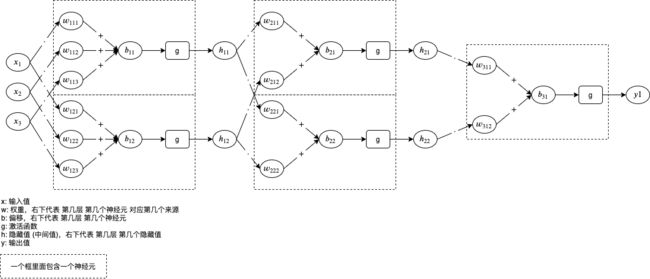
神经元中包含的 w 和 b 就是我们需要通过机器学习调整的参数值。
如果你觉得图片有点难以理解,可以看转换后的代码:
h11 = g(x1 * w111 + x2 * w112 + x3 * w113 + b11)
h12 = g(x1 * w121 + x2 * w122 + x3 * w123 + b12)
h21 = g(h11 * w211 + h12 * w212 + b21)
h22 = g(h11 * w221 + h12 * w222 + b22)
y = g(h21 * w311 + h22 * w312 + b31)
很多痴迷人工神经元网络的学者声称人工神经元网络可以模拟人脑的工作方式,做到某些领域上超过人脑的判断,但实际上这还有很大的争议,我们可以看到人工神经元的连接方式只会按固定的模式,判断是否达到阈值并输出的逻辑也无法做到和生物神经元一样(目前还没有解明),并且也没有生物神经元的不应期,所以也有学者声称人工神经元不过只是做了复杂的数学运算来模拟逻辑判断,需要根据不同的场景切换不同的计算方法,使用这种方式并不能达到人脑的水平。
4.2.单层线性模型
在前一篇文章我们已经稍微了解过机器学习框架 pytorch,现在我们来看看怎么使用 pytorch 封装的线性模型,以下代码运行在 python 的 REPL 中:
# 导入 pytorch 类库
>>> import torch

# 创建 pytorch 封装的线性模型,设置输入有 3 个输出有 1 个
>>> model = torch.nn.Linear(in_features=3, out_features=1)

# 查看线性模型内部包含的参数列表
# 这里一共包含两个参数,第一个参数是 1 行 3 列的矩阵分别表示 3 个输入对应的 w 值 (权重),第二个参数表示 b 值 (偏移)
# 初始值会随机生成 (使用 kaiming_uniform 生成正态分布)
>>> list(model.parameters())
[Parameter containing:
tensor([[0.0599, 0.1324, 0.0099]], requires_grad=True), Parameter containing:
tensor([-0.2772], requires_grad=True)]

# 定义输入和输出
>>> x = torch.tensor([1, 2, 3], dtype=torch.float)
>>> y = torch.tensor([6], dtype=torch.float)

# 把输入传给模型
>>> p = model(x)

# 查看预测输出值
# 1 * 0.0599 + 2 * 0.1324 + 3 * 0.0099 - 0.2772 = 0.0772
>>> p
tensor([0.0772], grad_fn=)

# 计算误差并自动微分
>>> l = (p - y).abs()
>>> l
tensor([5.9228], grad_fn=)
>>> l.backward()

# 查看各个参数对应的导函数值
>>> list(model.parameters())[0].grad
tensor([[-1., -2., -3.]])
>>> list(model.parameters())[1].grad
tensor([-1.])
以上可以看作 1 层 1 个神经元,很好理解吧?我们来看看 1 层 2 个神经元:
# 导入 pytorch 类库
>>> import torch

# 创建 pytorch 封装的线性模型,设置输入有 3 个输出有 2 个
>>> model = torch.nn.Linear(in_features=3, out_features=2)

# 查看线性模型内部包含的参数列表
# 这里一共包含两个参数
# 第一个参数是 2 行 3 列的矩阵分别表示 2 个输出和 3 个输入对应的 w 值 (权重)
# 第二个参数表示 2 个输出对应的 b 值 (偏移)
>>> list(model.parameters())
[Parameter containing:
tensor([[0.1393, 0.5165, 0.2910],
        [0.2276, 0.1579, 0.1958]], requires_grad=True), Parameter containing:
tensor([0.2566, 0.1701], requires_grad=True)]

# 定义输入和输出
>>> x = torch.tensor([1, 2, 3], dtype=torch.float)
>>> y = torch.tensor([6, -6], dtype=torch.float)

# 把输入传给模型
>>> p = model(x)

# 查看预测输出值
# 1 * 0.1393 + 2 * 0.5165 + 3 * 0.2910 + 0.2566 = 2.3019
# 1 * 0.2276 + 2 * 0.1579 + 3 * 0.1958 + 0.1701 = 1.3009
>>> p
tensor([2.3019, 1.3009], grad_fn=)

# 计算误差并自动微分
# (abs(2.3019 - 6) + abs(1.3009 - -6)) / 2 = 5.4995
>>> l = (p - y).abs().mean()
>>> l
tensor(5.4995, grad_fn=)
>>> l.backward()

# 查看各个参数对应的导函数值
# 因为误差取了 2 个值的平均,所以求导函数值的时候会除以 2
>>> list(model.parameters())[0].grad
tensor([[-0.5000, -1.0000, -1.5000],
        [ 0.5000,  1.0000,  1.5000]])
>>> list(model.parameters())[1].grad
tensor([-0.5000,  0.5000])
现在我们来试试用线性模型来学习符合 x_1 * 1 + x_2 * 2 + x_3 * 3 + 8 = y 的数据,输入和输出会使用矩阵定义:
# 引用 pytorch
import torch

# 给随机数生成器分配一个初始值,使得每次运行都可以生成相同的随机数
# 这是为了让训练过程可重现,你也可以选择不这样做
torch.random.manual_seed(0)

# 创建线性模型,设置有 3 个输入 1 个输出
model = torch.nn.Linear(in_features=3, out_features=1)

# 创建损失计算器
loss_function = torch.nn.MSELoss()

# 创建参数调整器
optimizer = torch.optim.SGD(model.parameters(), lr=0.01)

# 随机生成原始数据集,一共 20 组数据,每条数据有 3 个输入
dataset_x = torch.randn((20, 3))
dataset_y = dataset_x.mm(torch.tensor([[1], [2], [3]], dtype=torch.float)) + 8
print(f"dataset_x: {dataset_x}")
print(f"dataset_y: {dataset_y}")

# 切分训练集 (12 组),验证集 (4 组) 和测试集 (4 组)
random_indices = torch.randperm(dataset_x.shape[0])
traning_indices = random_indices[:int(len(random_indices)*0.6)]
validating_indices = random_indices[int(len(random_indices)*0.6):int(len(random_indices)*0.8):]
testing_indices = random_indices[int(len(random_indices)*0.8):]
traning_set_x = dataset_x[traning_indices]
traning_set_y = dataset_y[traning_indices]
validating_set_x = dataset_x[validating_indices]
validating_set_y = dataset_y[validating_indices]
testing_set_x = dataset_x[testing_indices]
testing_set_y = dataset_y[testing_indices]

# 开始训练过程
for epoch in range(1, 10000):
    print(f"epoch: {epoch}")

    # 根据训练集训练并修改参数
    # 切换模型到训练模式,将会启用自动微分,批次正规化 (BatchNorm) 与 Dropout
    model.train()

    # 计算预测值
    # 20 行 3 列的矩阵乘以 3 行 1 列的矩阵 (由 weight 转置得到) 等于 20 行 1 列的矩阵
    predicted = model(traning_set_x)
    # 计算损失
    loss = loss_function(predicted, traning_set_y)
    # 打印除错信息
    print(f"loss: {loss}, weight: {model.weight}, bias: {model.bias}")
    # 从损失自动微分求导函数值
    loss.backward()
    # 使用参数调整器调整参数
    optimizer.step()
    # 清空导函数值
    optimizer.zero_grad()

    # 检查验证集
    # 切换模型到验证模式,将会禁用自动微分,批次正规化 (BatchNorm) 与 Dropout
    model.eval()
    predicted = model(validating_set_x)
    validating_accuracy = 1 - ((validating_set_y - predicted).abs() / validating_set_y).abs().mean()
    print(f"validating x: {validating_set_x}, y: {validating_set_y}, predicted: {predicted}")

    # 如果验证集正确率大于 99 %,则停止训练
    print(f"validating accuracy: {validating_accuracy}")
    if validating_accuracy > 0.99:
        break

# 检查测试集
predicted = model(testing_set_x)
testing_accuracy = 1 - ((testing_set_y - predicted).abs() / testing_set_y).abs().mean()
print(f"testing x: {testing_set_x}, y: {testing_set_y}, predicted: {predicted}")
print(f"testing accuracy: {testing_accuracy}")
输出结果如下:
dataset_x: tensor([[ 0.8487, 0.6920, -0.3160],
[-2.1152, -0.3561, 0.4372],
[ 0.4913, -0.2041, 0.1198],
[ 1.2377, 1.1168, -0.2473],
[-1.0438, -1.3453, 0.7854],
[ 0.9928, 0.5988, -1.5551],
[-0.3414, 1.8530, 0.4681],
[-0.1577, 1.4437, 0.2660],
[ 1.3894, 1.5863, 0.9463],
[-0.8437, 0.9318, 1.2590],
[ 2.0050, 0.0537, 0.4397],
[ 0.1124, 0.6408, 0.4412],
[-0.2159, -0.7425, 0.5627],
[ 0.2596, 0.5229, 2.3022],
[-1.4689, -1.5867, -0.5692],
[ 0.9200, 1.1108, 1.2899],
[-1.4782, 2.5672, -0.4731],
[ 0.3356, -1.6293, -0.5497],
[-0.4798, -0.4997, -1.0670],
[ 1.1149, -0.1407, 0.8058]])
dataset_y: tensor([[ 9.2847],
[ 6.4842],
[ 8.4426],
[10.7294],
[ 6.6217],
[ 5.5252],
[12.7689],
[11.5278],
[15.4009],
[12.7970],
[11.4315],
[10.7175],
[ 7.9872],
[16.2120],
[ 1.6500],
[15.0112],
[10.2369],
[ 3.4277],
[ 3.3199],
[11.2509]])
epoch: 1
loss: 142.77590942382812, weight: Parameter containing:
tensor([[-0.0043, 0.3097, -0.4752]], requires_grad=True), bias: Parameter containing:
tensor([-0.4249], requires_grad=True)
validating x: tensor([[-0.4798, -0.4997, -1.0670],
[ 0.8487, 0.6920, -0.3160],
[ 0.1124, 0.6408, 0.4412],
[-1.0438, -1.3453, 0.7854]]), y: tensor([[ 3.3199],
[ 9.2847],
[10.7175],
[ 6.6217]]), predicted: tensor([[-0.1385],
[ 0.3020],
[-0.0126],
[-1.1801]], grad_fn=)
validating accuracy: -0.04714548587799072
epoch: 2
loss: 131.40403747558594, weight: Parameter containing:
tensor([[ 0.0675, 0.4937, -0.3163]], requires_grad=True), bias: Parameter containing:
tensor([-0.1970], requires_grad=True)
validating x: tensor([[-0.4798, -0.4997, -1.0670],
[ 0.8487, 0.6920, -0.3160],
[ 0.1124, 0.6408, 0.4412],
[-1.0438, -1.3453, 0.7854]]), y: tensor([[ 3.3199],
[ 9.2847],
[10.7175],
[ 6.6217]]), predicted: tensor([[-0.2023],
[ 0.6518],
[ 0.3935],
[-1.1479]], grad_fn=)
validating accuracy: -0.03184401988983154
epoch: 3
loss: 120.98343658447266, weight: Parameter containing:
tensor([[ 0.1357, 0.6687, -0.1639]], requires_grad=True), bias: Parameter containing:
tensor([0.0221], requires_grad=True)
validating x: tensor([[-0.4798, -0.4997, -1.0670],
[ 0.8487, 0.6920, -0.3160],
[ 0.1124, 0.6408, 0.4412],
[-1.0438, -1.3453, 0.7854]]), y: tensor([[ 3.3199],
[ 9.2847],
[10.7175],
[ 6.6217]]), predicted: tensor([[-0.2622],
[ 0.9860],
[ 0.7824],
[-1.1138]], grad_fn=)
validating accuracy: -0.016991496086120605省略途中输出
epoch: 637
loss: 0.001102567883208394, weight: Parameter containing:
tensor([[1.0044, 2.0283, 3.0183]], requires_grad=True), bias: Parameter containing:
tensor([7.9550], requires_grad=True)
validating x: tensor([[-0.4798, -0.4997, -1.0670],
[ 0.8487, 0.6920, -0.3160],
[ 0.1124, 0.6408, 0.4412],
[-1.0438, -1.3453, 0.7854]]), y: tensor([[ 3.3199],
[ 9.2847],
[10.7175],
[ 6.6217]]), predicted: tensor([[ 3.2395],
[ 9.2574],
[10.6993],
[ 6.5488]], grad_fn=)
validating accuracy: 0.9900396466255188
testing x: tensor([[-0.3414, 1.8530, 0.4681],
[-1.4689, -1.5867, -0.5692],
[ 1.1149, -0.1407, 0.8058],
[ 0.3356, -1.6293, -0.5497]]), y: tensor([[12.7689],
[ 1.6500],
[11.2509],
[ 3.4277]]), predicted: tensor([[12.7834],
[ 1.5438],
[11.2217],
[ 3.3285]], grad_fn=)
testing accuracy: 0.9757462739944458
可以看到最终 weight 接近 1, 2, 3,bias 接近 8。和前一篇文章最后的例子比较还可以发现代码除了定义模型的部分以外几乎一模一样 (后面的代码基本上都是相同的结构,这个系列是先学套路在学细节) 。
看到这里你可能会觉得,怎么我们一直都在学习一次方程式,不能做更复杂的事情吗?
如我们看到的,线性模型只能计算一次方程式,如果我们给的数据不满足任何一次方程式,这个模型将无法学习成功,那么叠加多层线性模型可以学习更复杂的数据吗?
以下是一层和两层人工神经元网络的公式例子:

因为我们还没有学到激活函数,先去掉激活函数,然后展开没有激活函数的两层人工神经元网络看看是什么样子:
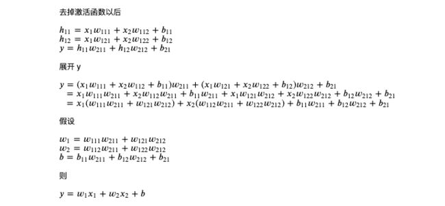
从上图可以看出,如果没有激活函数,两层人工神经元网络和一层神经元网络效果是一样的,实际上,如果没有激活函数不管叠加多少层都和一层一样,所以如果我们要构建多层网络,必须添加激活函数。
4.3.激活函数
激活函数的作用是让人工神经元网络支持学习非线性的数据,所谓非线性的数据就是不满足任何一次方程式的数据,输出和输入之间不会按一定比例变化。举个很简单的例子,如果需要按码农的数量计算某个项目所需的完工时间,一个码农需要一个月,两个码农需要半个月,三个码农需要十天,四个码农需要一个星期,之后无论请多少个码农都需要一个星期,多出来的码农只会吃闲饭,使用图表可以表现如下:
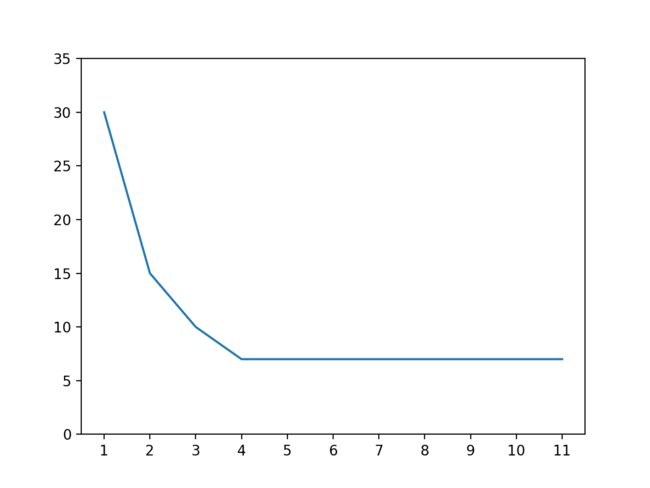
如果不用激活函数,只用线性模型可以调整 w 到 -5.4,b 到 30,使用图表对比 -5.4 x + 30 和实际数据如下,我们可以看到不仅预测的误差较大,随着码农数量的增长预测所需的完工时间会变为负数:
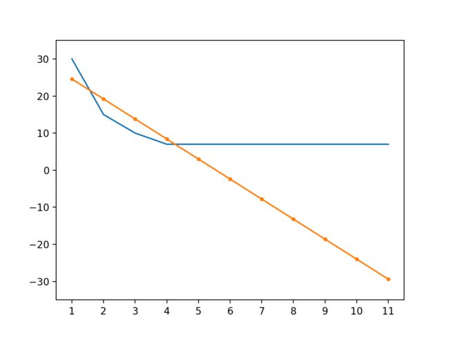
那么使用激活函数会怎样呢?我们以最简单也是最流行的激活函数 ReLU (Rectified Linear Unit) 为例,ReLU 函数的定义如下:

意思是传入值大于 0 时返回原值,否则返回 0,用 python 代码可以表现如下:
def relu(x):
    if x > 0:
        return x
    return 0
再看看以下结合了 ReLU 激活函数的两层人工神经元网络 (最后一层不使用激活函数):

试试计算上面的例子:
def relu(x):
    if x > 0:
        return x
    return 0

for x in range(1, 11):
    h1 = relu(x * -1 + 2)
    h2 = relu(x * -1 + 3)
    h3 = relu(x * -1 + 4)
    y = h1 * 10 + h2 * 2 + h3 * 3 + 7
    print(x, y)
输入如下,可以看到添加激活函数后模型能够支持计算上面的非线性数据:
1 30
2 15
3 10
4 7
5 7
6 7
7 7
8 7
9 7
10 7
激活函数除了上述介绍的 ReLU 还有很多,以下是一些常用的激活函数:

如果你想看它们的曲线和导函数可以参考以下链接:
- torch.nn — PyTorch 1.12 documentation
- Activation Functions — ML Glossary documentation
添加激活函数以后求导函数值同样可以使用连锁律,如果第一层返回的是正数,那么就和没有 ReLU 时的计算一样 (导函数为 1):
>>> w1 = torch.tensor(5.0, requires_grad=True)
>>> b1 = torch.tensor(1.0, requires_grad=True)
>>> w2 = torch.tensor(6.0, requires_grad=True)
>>> b2 = torch.tensor(7.0, requires_grad=True)

>>> x = torch.tensor(2.0)
>>> y = torch.nn.functional.relu(x * w1 + b1) * w2 + b2

# 假设我们要调整 w1, b1, w2, b2 使得 y 接近 0
>>> y
tensor(73., grad_fn=)
>>> y.abs().backward()

# w1 的导函数值为 x * w2
>>> w1.grad
tensor(12.)

# b1 的导函数值为 w2
>>> b1.grad
tensor(6.)

# w2 的导函数值为 x * w1 + b1
>>> w2.grad
tensor(11.)

# b1 的导函数值为 1
>>> b2.grad
tensor(1.)
假设第一层返回的是负数,那么 ReLU 会让上一层的导函数值为 0 (导函数为 0):
>>> w1 = torch.tensor(5.0, requires_grad=True)
>>> b1 = torch.tensor(1.0, requires_grad=True)
>>> w2 = torch.tensor(6.0, requires_grad=True)
>>> b2 = torch.tensor(7.0, requires_grad=True)

>>> x = torch.tensor(-2.0)
>>> y = torch.nn.functional.relu(x * w1 + b1) * w2 + b2

>>> y
tensor(7., grad_fn=)
>>> y.backward()

>>> w1.grad
tensor(-0.)
>>> b1.grad
tensor(0.)
>>> w2.grad
tensor(0.)
>>> b2.grad
tensor(1.)
虽然 ReLU 可以适合大部分场景,但有时候我们还是需要选择其他激活函数,选择激活函数一般会考虑以下的因素:
- 计算量
- 是否存在梯度消失 (Vanishing Gradient) 问题
- 是否存在停止学习问题
从上图我们可以看到 ReLU 的计算量是最少的,Sigmoid 和 Tanh 的计算量则很大,使用计算量大的激活函数会导致学习过程更慢。
而梯度消失 (Vanishing Gradient) 问题则是在人工神经元网络层数增多以后出现的问题,如果层数不断增多,使用连锁律求导函数的时候会不断叠加激活函数的导函数,部分激活函数例如 Sigmoid 和 Tanh 的导函数会随着叠加次数增多而不断的减少导函数值。例如有 3 层的时候,第 3 层导函数值可能是 6, -2, 1,第 2 层的导函数值可能是 0.07, 0.68, -0.002,第 1 层的导函数值可能是 0.0004, -0.00016, -0.00003,也就是前面的层参数基本上不会调整,只有后面的层参数不断变化,导致浪费计算资源和不能完全发挥模型的能力。激活函数 ReLU 则不会存在梯度消失问题,因为不管叠加多少层只要中间不存在负数则导函数值会一直传递上去,这也是 ReLU 流行的原因之一。
停止学习问题是模型达到某个状态 (未学习成功) 以后不管怎么调整参数都不会变化的问题,一个简单的例子是使用 ReLU 时,如果第一层的输出刚好全部都是负数,那隐藏值则全部为 0,导函数值也为 0,不管再怎么训练参数都不会变化。LeakyReLU 与 ELU 则是为了解决停止学习问题产生的,但因为增加计算量和允许负数可能会带来其他影响,我们一般都会先使用 ReLU,出现停止学习问题再试试 ReLU 的派生函数。
Sigmoid 和 Tanh 虽然有梯度消失问题,但是它们可以用于在指定场景下转换数值到 0 ~ 1 和 -1 ~ 1。例如 Sigmoid 可以用在最后一层表现可能性,100 表示非常有可能 (转换到 1),50 也代表非常有可能 (转换到 1),1 代表比较有可能 (转换到 0.7311),0 代表不确定 (转换到 0.5),-1 代表比较不可能 (转换到 0.2689),-100 代表很不可能 (转换到 0)。而后面文章介绍的 LSTM 模型也会使用 Sigmoid 决定需要忘记哪些内部状态,Tanh 决定应该怎样更新内部状态。此外还有 Softmax 等一般只用在最后一层的函数,Softmax 可以用于在分类的时候判断哪个类别可能性最大,例如识别猫狗猪的时候最后一层给出 6, 5, 8,数值越大代表属于该分类的可能性越高,经过 Softmax 转换以后就是 0.1142, 0.0420, 0.8438,代表有 11.42% 的可能性是猫,4.2% 的可能性是狗,84.38% 的可能性是猪。
4.4.多层线性模型
接下来我们看看怎样在 pytorch 里面定义多层线性模型,上一节已经介绍过 torch.nn.Linear 是 pytorch 中单层线性模型的封装,组合多个 torch.nn.Linear 就可以实现多层线性模型。
组合 torch.nn.Linear 有两种方法,一种创建一个自定义的模型类,关于模型类在上一篇已经介绍过:
# 引用 pytorch,nn 等同于 torch.nn
import torch
from torch import nn

# 定义模型
class MyModel(nn.Module):
    def __init__(self):
        # 初始化基类
        super().__init__()
        # 定义参数
        # 这里一共定义了三层
        #   第一层接收 2 个输入,返回 32 个隐藏值 (内部 weight 矩阵为 32 行 2 列)
        #   第二层接收 32 个隐藏值,返回 64 个隐藏值 (内部 weight 矩阵为 64 行 32 列)
        #   第三层接收 64 个隐藏值,返回 1 个输出 (内部 weight 矩阵为 1 行 64 列)
        self.layer1 = nn.Linear(in_features=2, out_features=32)
        self.layer2 = nn.Linear(in_features=32, out_features=64)
        self.layer3 = nn.Linear(in_features=64, out_features=1)

    def forward(self, x):
        # x 是一个矩阵,行数代表批次,列数代表输入个数,例如有 50 个批次则为 50 行 2 列

        # 计算第一层返回的隐藏值,例如有 50 个批次则 hidden1 为 50 行 32 列
        # 计算矩阵乘法时会转置 layer1 内部的 weight 矩阵,50 行 2 列乘以 2 行 32 列等于 50 行 32 列
        hidden1 = nn.functional.relu(self.layer1(x))

        # 计算第二层返回的隐藏值,例如有 50 个批次则 hidden2 为 50 行 64 列
        hidden2 = nn.functional.relu(self.layer2(hidden1))

        # 计算第三层返回的输出,例如有 50 个批次则 y 为 50 行 1 列
        y = self.layer3(hidden2)

        # 返回输出
        return y

# 创建模型实例
model = MyModel()
我们可以定义任意数量的层,但每一层的接收值个数 (in_features) 必须等于上一层的返回值个数 (out_features),第一层的接收值个数需要等于输入个数,最后一层的返回值个数需要等于输出个数。
第二种方法是使用 torch.nn.Sequential,这种方法更简便:
# 引用 pytorch,nn 等同于 torch.nn
import torch
from torch import nn

# 创建模型实例,效果等同于第一种方法
model = nn.Sequential(
    nn.Linear(in_features=2, out_features=32),
    nn.ReLU(),
    nn.Linear(in_features=32, out_features=64),
    nn.ReLU(),
    nn.Linear(in_features=64, out_features=1))

# 注:
# nn.functional.relu(x) 等于 nn.ReLU()(x)
如前面所说的,层数越多隐藏值数量越多模型就越强大,但需要更长的训练时间并且更容易发生过拟合问题,实际操作时我们可以选择一个比较小的模型,再按需要增加层数和隐藏值个数。
三层线性模型的计算图可以表现如下,以后这个系列在讲解其他模型的时候也会使用相同形式的图表表示模型的计算路径:

4.5.根据码农条件求工资
我们已经了解到如何创建多层线性模型,现在可以试试解决比较实际的问题了,对于大部分码农来说最实际的问题就是每个月能拿多少工资,那就来建立一个根据码农的条件,预测可以拿到多少工资的模型吧。
以下是从某个地方秘密收集回来的码农条件和工资数据(其实是按某种规律随机生成出来的,不是实际数据):
年龄,性别,工作经验,Java,NET,JS,CSS,HTML,工资
29,0,0,1,2,2,1,4,12500
22,0,2,2,3,1,2,5,15500
24,0,4,1,2,1,1,2,16000
35,0,6,3,3,0,1,0,19500
45,0,18,0,5,2,0,5,17000
24,0,2,0,0,0,1,1,13500
23,1,2,2,3,1,1,0,10500
41,0,16,2,5,5,2,0,16500
50,0,18,0,5,0,5,2,16500
20,0,0,0,5,2,0,1,12500
26,0,6,1,5,5,1,1,27000
46,0,12,0,5,4,4,2,12500
26,0,6,1,5,3,1,1,23500
40,0,9,0,0,1,0,1,17500
41,0,20,3,5,3,3,5,20500
26,0,4,0,1,2,4,0,18500
42,0,18,5,0,0,2,5,18500
21,0,1,1,0,1,2,0,12000
26,0,1,0,0,0,0,2,12500
完整数据有 50000 条,可以从 303248153.github.io/salary.csv at master · 303248153/303248153.github.io · GitHub 下载。
每个码农有以下条件:
- 年龄
- 性别 (0: 男性, 1: 女性)
- 工作经验年数 (仅限互联网行业)
- Java 编码熟练程度 (0 ~ 5)
- NET 编码熟练程度 (0 ~ 5)
- JS 编码熟练程度 (0 ~ 5)
- CSS 编码熟练程度 (0 ~ 5)
- HTML 编码熟练程度 (0 ~ 5)
也就是有 8 个输入,1 个输出 (工资),我们可以建立三层线性模型:
- 第一层接收 8 个输入返回 100 个隐藏值
- 第二层接收 100 个隐藏值返回 50 个隐藏值
- 第三层接收 50 个隐藏值返回 1 个输出
写成代码如下 (这里使用了 pandas 类库读取 csv,使用 pip3 install pandas 即可安装):
# 引用 pytorch 和 pandas
import pandas
import torch
from torch import nn

# 定义模型
class MyModel(nn.Module):
    def __init__(self):
        super().__init__()
        self.layer1 = nn.Linear(in_features=8, out_features=100)
        self.layer2 = nn.Linear(in_features=100, out_features=50)
        self.layer3 = nn.Linear(in_features=50, out_features=1)

    def forward(self, x):
        hidden1 = nn.functional.relu(self.layer1(x))
        hidden2 = nn.functional.relu(self.layer2(hidden1))
        y = self.layer3(hidden2)
        return y

# 给随机数生成器分配一个初始值,使得每次运行都可以生成相同的随机数
# 这是为了让训练过程可重现,你也可以选择不这样做
torch.random.manual_seed(0)

# 创建模型实例
model = MyModel()

# 创建损失计算器
loss_function = torch.nn.MSELoss()

# 创建参数调整器
optimizer = torch.optim.SGD(model.parameters(), lr=0.0000001)

# 从 csv 读取原始数据集
df = pandas.read_csv('salary.csv')
dataset_tensor = torch.tensor(df.values, dtype=torch.float)

# 切分训练集 (60%),验证集 (20%) 和测试集 (20%)
random_indices = torch.randperm(dataset_tensor.shape[0])
traning_indices = random_indices[:int(len(random_indices)*0.6)]
validating_indices = random_indices[int(len(random_indices)*0.6):int(len(random_indices)*0.8):]
testing_indices = random_indices[int(len(random_indices)*0.8):]
traning_set_x = dataset_tensor[traning_indices][:,:-1]
traning_set_y = dataset_tensor[traning_indices][:,-1:]
validating_set_x = dataset_tensor[validating_indices][:,:-1]
validating_set_y = dataset_tensor[validating_indices][:,-1:]
testing_set_x = dataset_tensor[testing_indices][:,:-1]
testing_set_y = dataset_tensor[testing_indices][:,-1:]

# 开始训练过程
for epoch in range(1, 1000):
    print(f"epoch: {epoch}")

    # 根据训练集训练并修改参数
    # 切换模型到训练模式,将会启用自动微分,批次正规化 (BatchNorm) 与 Dropout
    model.train()

    for batch in range(0, traning_set_x.shape[0], 100):
        # 切分批次,一次只计算 100 组数据
        batch_x = traning_set_x[batch:batch+100]
        batch_y = traning_set_y[batch:batch+100]
        # 计算预测值
        predicted = model(batch_x)
        # 计算损失
        loss = loss_function(predicted, batch_y)
        # 从损失自动微分求导函数值
        loss.backward()
        # 使用参数调整器调整参数
        optimizer.step()
        # 清空导函数值
        optimizer.zero_grad()

    # 检查验证集
    # 切换模型到验证模式,将会禁用自动微分,批次正规化 (BatchNorm) 与 Dropout
    model.eval()
    predicted = model(validating_set_x)
    validating_accuracy = 1 - ((validating_set_y - predicted).abs() / validating_set_y).mean()
    print(f"validating x: {validating_set_x}, y: {validating_set_y}, predicted: {predicted}")
    print(f"validating accuracy: {validating_accuracy}")

# 检查测试集
predicted = model(testing_set_x)
testing_accuracy = 1 - ((testing_set_y - predicted).abs() / testing_set_y).mean()
print(f"testing x: {testing_set_x}, y: {testing_set_y}, predicted: {predicted}")
print(f"testing accuracy: {testing_accuracy}")

# 手动输入数据预测输出
while True:
    try:
        print("enter input:")
        r = list(map(float, input().split(",")))
        x = torch.tensor(r).view(1, len(r))
        print(model(x)[0,0].item())
    except Exception as e:
        print("error:", e)
输出如下,可以看到最后没有参与训练的验证集的正确度达到了 93.3% 测试集的正确度达到了 93.1%,模型成功的摸索出了某种规律:
epoch: 1
validating x: tensor([[42., 0., 16., ..., 5., 5., 5.],
[28., 0., 0., ..., 4., 0., 0.],
[23., 0., 3., ..., 0., 1., 1.],
...,
[44., 1., 15., ..., 2., 0., 2.],
[30., 0., 1., ..., 1., 1., 2.],
[50., 1., 18., ..., 5., 5., 2.]]), y: tensor([[24500.],
[12500.],
[17500.],
...,
[10500.],
[15000.],
[16000.]]), predicted: tensor([[27604.2578],
[15934.7607],
[14536.8984],
...,
[23678.5547],
[18189.6953],
[29968.8789]], grad_fn=)
validating accuracy: 0.661293625831604
epoch: 2
validating x: tensor([[42., 0., 16., ..., 5., 5., 5.],
[28., 0., 0., ..., 4., 0., 0.],
[23., 0., 3., ..., 0., 1., 1.],
...,
[44., 1., 15., ..., 2., 0., 2.],
[30., 0., 1., ..., 1., 1., 2.],
[50., 1., 18., ..., 5., 5., 2.]]), y: tensor([[24500.],
[12500.],
[17500.],
...,
[10500.],
[15000.],
[16000.]]), predicted: tensor([[29718.2441],
[15790.3799],
[15312.5791],
...,
[23395.9668],
[18672.0234],
[31012.4062]], grad_fn=)
validating accuracy: 0.6694601774215698省略途中输出
epoch: 999
validating x: tensor([[42., 0., 16., ..., 5., 5., 5.],
[28., 0., 0., ..., 4., 0., 0.],
[23., 0., 3., ..., 0., 1., 1.],
...,
[44., 1., 15., ..., 2., 0., 2.],
[30., 0., 1., ..., 1., 1., 2.],
[50., 1., 18., ..., 5., 5., 2.]]), y: tensor([[24500.],
[12500.],
[17500.],
...,
[10500.],
[15000.],
[16000.]]), predicted: tensor([[22978.7656],
[13050.8018],
[18396.5176],
...,
[11449.5059],
[14791.2969],
[16635.2578]], grad_fn=)
validating accuracy: 0.9311849474906921
testing x: tensor([[48., 1., 18., ..., 5., 0., 5.],
[22., 1., 2., ..., 2., 1., 2.],
[24., 0., 1., ..., 3., 2., 0.],
...,
[24., 0., 4., ..., 0., 1., 1.],
[39., 0., 0., ..., 0., 5., 5.],
[36., 0., 5., ..., 3., 0., 3.]]), y: tensor([[14000.],
[10500.],
[13000.],
...,
[15500.],
[12000.],
[19000.]]), predicted: tensor([[15481.9062],
[11011.7266],
[12192.7949],
...,
[16219.3027],
[11074.0420],
[20305.3516]], grad_fn=)
testing accuracy: 0.9330180883407593
enter input:
最后我们手动输入码农条件可以得出预测输出 (35 岁男 10 年经验 Java 5 NET 2 JS 1 CSS 1 HTML 2 大约可拿 26k ):
enter input:
35,0,10,5,2,1,1,2
26790.982421875
虽然训练成功了,但以上代码还有几个问题:
- 学习比率设置的非常低 (0.0000001),这是因为我们没有对数据进行正规化处理
- 总是会固定训练 1000 次,不能像第一篇文章提到过的那样自动检测哪一次的正确度最高,没有考虑过拟合问题
- 不能把训练结果保存到硬盘,每次运行都需要从头训练
- 需要把所有数据一次性读取到内存中,数据过多时内存可能不够用
- 没有提供一个使用训练好的模型的接口
这些问题都会在下篇文章一个个解决。