回归分析代码实现

1.statsmodel回归分析

import numpy as np
import matplotlib.pyplot as plt
import statsmodels.api as sm

nsample = 20
x = np.linspace(0, 10, nsample)
x

 

#一元线性回归 
X = sm.add_constant(x)
X

#β0,β1分别设置成2,5
beta = np.array([2, 5])
beta

 

#误差项
e = np.random.normal(size=nsample)
e

#实际值y
y = np.dot(X, beta) + e
y

 

#最小二乘法
model = sm.OLS(y,X)

#拟合数据
res = model.fit()

#回归系数
res.params
>>>array([ 1.49524076,  5.08701837])

#全部结果
res.summary()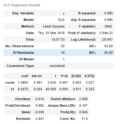

 

#拟合的估计值
y_ = res.fittedvalues
y_

 

fig, ax = plt.subplots(figsize=(8,6))
ax.plot(x, y, 'o', label='data')#原始数据
ax.plot(x, y_, 'r--.',label='test')#拟合数据
ax.legend(loc='best')
plt.show()

 

2.高阶回归和分类变量

高阶回归

#Y=5+2⋅X+3⋅X^2
 
nsample = 50
x = np.linspace(0, 10, nsample)
X = np.column_stack((x, x**2))
X = sm.add_constant(X)

beta = np.array([5, 2, 3])
e = np.random.normal(size=nsample)
y = np.dot(X, beta) + e
model = sm.OLS(y,X)
results = model.fit()
results.params

>>> array([ 4.93210623,  2.16604081,  2.97682135])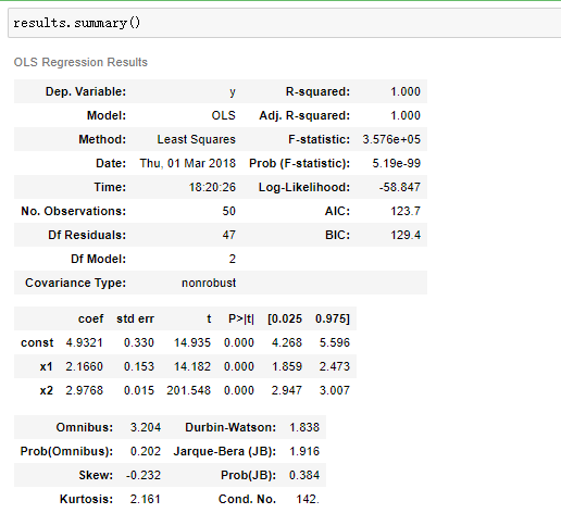

 

y_fitted = results.fittedvalues
fig, ax = plt.subplots(figsize=(8,6))
ax.plot(x, y, 'o', label='data')
ax.plot(x, y_fitted, 'r--.',label='OLS')
ax.legend(loc='best')
plt.show()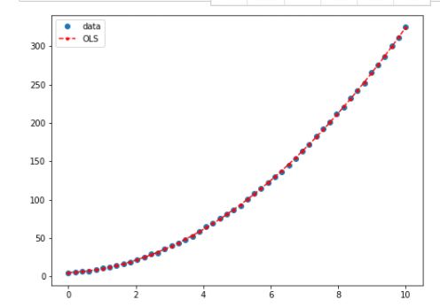

 

分类变量 

        假设分类变量有4个取值（a,b,c）,比如考试成绩有3个等级。那么a就是（1,0,0），b（0,1,0），c(0,0,1),这个时候就需要3个系数β0,β1,β2，也就是β0x0+β1x1+β2x2

nsample = 50
groups = np.zeros(nsample,int)
groups

groups[20:40] = 1
groups[40:] = 2
dummy = sm.categorical(groups, drop=True)
dummy 

 

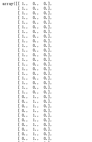
#Y=5+2X+3Z1+6⋅Z2+9⋅Z3.
 
x = np.linspace(0, 20, nsample)
X = np.column_stack((x, dummy))
X = sm.add_constant(X)
beta = [5, 2, 3, 6, 9]
e = np.random.normal(size=nsample)
y = np.dot(X, beta) + e
result = sm.OLS(y,X).fit()
result.summary()

 

fig, ax = plt.subplots(figsize=(8,6))
ax.plot(x, y, 'o', label="data")
ax.plot(x, result.fittedvalues, 'r--.', label="OLS")
ax.legend(loc='best')
plt.show()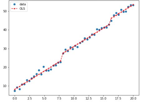

 

 

 2.实例：汽车价格预测

数据集简介

主要包括3类指标:

• 汽车的各种特性.
• 保险风险评级：(-3, -2, -1, 0, 1, 2, 3).
• 每辆保险车辆年平均相对损失支付.

类别属性

• make: 汽车的商标（奥迪，宝马。。。）
• fuel-type: 汽油还是天然气
• aspiration: 涡轮
• num-of-doors: 两门还是四门
• body-style: 硬顶车、轿车、掀背车、敞篷车
• drive-wheels: 驱动轮
• engine-location: 发动机位置
• engine-type: 发动机类型
• num-of-cylinders: 几个气缸
• fuel-system: 燃油系统

连续指标

• bore: continuous from 2.54 to 3.94.
• stroke: continuous from 2.07 to 4.17.
• compression-ratio: continuous from 7 to 23.
• horsepower: continuous from 48 to 288.
• peak-rpm: continuous from 4150 to 6600.
• city-mpg: continuous from 13 to 49.
• highway-mpg: continuous from 16 to 54.
• price: continuous from 5118 to 45400.

数据读取与分析

# loading packages
import numpy as np
import pandas as pd
from pandas import datetime

# data visualization and missing values
import matplotlib.pyplot as plt
import seaborn as sns # advanced vizs
import missingno as msno # missing values
%matplotlib inline

# stats
from statsmodels.distributions.empirical_distribution import ECDF
from sklearn.metrics import mean_squared_error, r2_score

# machine learning
from sklearn.preprocessing import StandardScaler
from sklearn.linear_model import Lasso, LassoCV 
from sklearn.model_selection import train_test_split, cross_val_score 
from sklearn.ensemble import RandomForestRegressor
seed = 123

# importing data ( ? = missing values)
data = pd.read_csv("Auto-Data.csv", na_values = '?')
data.columns

 

 

# first glance at the data itself
print("In total: ",data.shape)
data.head(5)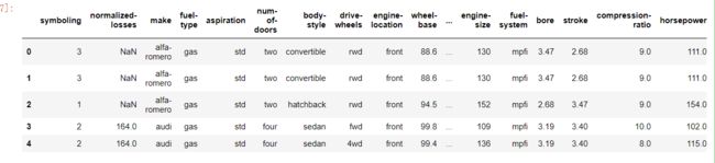

 

 

缺失值处理 

# missing values?
sns.set(style = "ticks")

msno.matrix(data)
#https://github.com/ResidentMario/missingno

 

# missing values in normalied-losses
data[pd.isnull(data['normalized-losses'])].head()

sns.set(style = "ticks")
plt.figure(figsize = (12, 5)) 
c = '#366DE8'

# ECDF
plt.subplot(121)
cdf = ECDF(data['normalized-losses'])
plt.plot(cdf.x, cdf.y, label = "statmodels", color = c);
plt.xlabel('normalized losses'); plt.ylabel('ECDF');

# overall distribution
plt.subplot(122)
plt.hist(data['normalized-losses'].dropna(), 
         bins = int(np.sqrt(len(data['normalized-losses']))),
         color = c);

 

可以发现 80% 的 normalized losses 是低于200 并且绝大多数低于125.数据严重偏态分布，因此，不适合用平均值来进行填充。

一个基本的想法就是用中位数来进行填充，但是我们得来想一想，这个特征跟哪些因素可能有关呢？应该是保险的情况吧，所以我们可以分组来进行填充这样会更精确一些。

 

对缺失值不多的直接删除 

# replacing
data = data.dropna(subset = ['price', 'bore', 'stroke', 'peak-rpm', 'horsepower', 'num-of-doors'])
data['normalized-losses'] = data.groupby('symboling')['normalized-losses'].transform(lambda x: x.fillna(x.mean()))

print('In total:', data.shape)
data.head()

 

特征相关性

cormatrix = data.corr()
cormatrix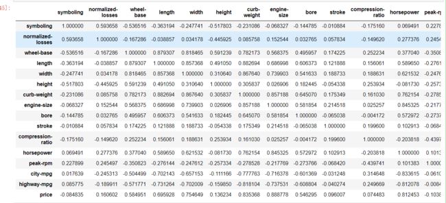

 

cormatrix *= np.tri(*cormatrix.values.shape, k=-1).T  #返回函数的上三角矩阵，
把对角线上的置0，让他们不是最高的。
cormatrix

 

cormatrix = cormatrix.stack()
cormatrix 

 

cormatrix = cormatrix.reindex(cormatrix.abs().sort_values(ascending=False).index).reset_index()
cormatrix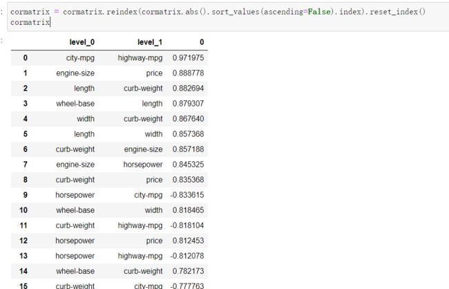

 

cormatrix.columns = ["FirstVariable", "SecondVariable", "Correlation"]
cormatrix.head(10)

 

city_mpg 和 highway-mpg 意思差不多. 对于这个长宽高，他们应该存在某种配对关系，给他们合体吧！ 

 

data['volume'] = data.length * data.width * data.height

data.drop(['width', 'length', 'height', 
           'curb-weight', 'city-mpg'], 
          axis = 1, # 1 for columns
          inplace = True) 

 

np.triu(arr,k) 返回矩阵的上三角矩阵，K值不同，矩阵会有所变化

np.triu_indices（arr,k）/np.triu_indices_from() 返回矩阵的索引 

# Compute the correlation matrix 
corr_all = data.corr()

# Generate a mask for the upper triangle
mask = np.zeros_like(corr_all, dtype = np.bool)
mask[np.triu_indices_from(mask)] = True

# Set up the matplotlib figure
f, ax = plt.subplots(figsize = (11, 9))

# Draw the heatmap with the mask and correct aspect ratio
sns.heatmap(corr_all, mask = mask,
            square = True, linewidths = .5, ax = ax, cmap = "BuPu")      
plt.show()

 

看起来 price 跟这几个的相关程度比较大 wheel-base,enginine-size, bore,horsepower.

sns.pairplot(data, hue = 'fuel-type', palette = 'plasma')

 

让我们仔细看看价格和马力变量之间的关系，指定特定行和列

sns.lmplot('price', 'horsepower', data, 
           hue = 'fuel-type', col = 'fuel-type',  row = 'num-of-doors', 
           palette = 'plasma', 
           fit_reg = True);

 

 

 预处理

如果一个特性的方差比其他的要大得多，那么它可能支配目标函数，使估计者不能像预期的那样正确地从其他特性中学习。这就是为什么我们需要首先对数据进行缩放。

对连续值进行标准化

# target and features
target = data.price

regressors = [x for x in data.columns if x not in ['price']]
features = data.loc[:, regressors]

num = ['symboling', 'normalized-losses', 'volume', 'horsepower', 'wheel-base',
       'bore', 'stroke','compression-ratio', 'peak-rpm']

# scale the data
standard_scaler = StandardScaler()
features[num] = standard_scaler.fit_transform(features[num])

# glimpse
features.head()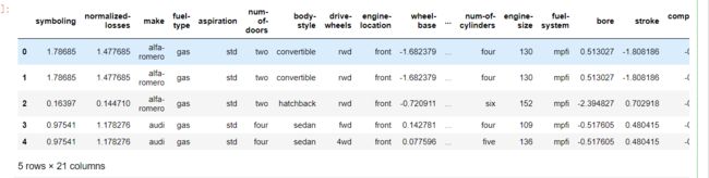

 

对分类属性就行one-hot编码

# categorical vars
classes = ['make', 'fuel-type', 'aspiration', 'num-of-doors', 
           'body-style', 'drive-wheels', 'engine-location',
           'engine-type', 'num-of-cylinders', 'fuel-system']

# create new dataset with only continios vars 
dummies = pd.get_dummies(features[classes])
features = features.join(dummies).drop(classes, 
                                       axis = 1)

# new dataset
print('In total:', features.shape)
features.head()

 

划分数据集

# split the data into train/test set
X_train, X_test, y_train, y_test = train_test_split(features, target, 
                                                    test_size = 0.3,
                                                    random_state = seed)
print("Train", X_train.shape, "and test", X_test.shape)

 3.回归求解

Lasso回归

# logarithmic scale: log base 2
# high values to zero-out more variables
alphas = 2. ** np.arange(2, 12)
scores = np.empty_like(alphas)

for i, a in enumerate(alphas):
    lasso = Lasso(random_state = seed)
    lasso.set_params(alpha = a)
    lasso.fit(X_train, y_train)
    scores[i] = lasso.score(X_test, y_test)
    
lassocv = LassoCV(cv = 10, random_state = seed)
lassocv.fit(features, target)
lassocv_score = lassocv.score(features, target)
lassocv_alpha = lassocv.alpha_

plt.figure(figsize = (10, 4))
plt.plot(alphas, scores, '-ko')
plt.axhline(lassocv_score, color = c)
plt.xlabel(r'$\alpha$')
plt.ylabel('CV Score')
plt.xscale('log', basex = 2)
sns.despine(offset = 15)

print('CV results:', lassocv_score, lassocv_alpha)

 

# lassocv coefficients
coefs = pd.Series(lassocv.coef_, index = features.columns)

# prints out the number of picked/eliminated features
print("Lasso picked " + str(sum(coefs != 0)) + " features and eliminated the other " +  \
      str(sum(coefs == 0)) + " features.")

# takes first and last 10
coefs = pd.concat([coefs.sort_values().head(5), coefs.sort_values().tail(5)])

plt.figure(figsize = (10, 4))
coefs.plot(kind = "barh", color = c)
plt.title("Coefficients in the Lasso Model")
plt.show()

 

model_l1 = LassoCV(alphas = alphas, cv = 10, random_state = seed).fit(X_train, y_train)
y_pred_l1 = model_l1.predict(X_test)

model_l1.score(X_test, y_test)

 >>> 0.83307445226244159

 

# residual plot
plt.rcParams['figure.figsize'] = (6.0, 6.0)

preds = pd.DataFrame({"preds": model_l1.predict(X_train), "true": y_train})
preds["residuals"] = preds["true"] - preds["preds"]
preds.plot(x = "preds", y = "residuals", kind = "scatter", color = c)

 

def MSE(y_true,y_pred):
    mse = mean_squared_error(y_true, y_pred)
    print('MSE: %2.3f' % mse)
    return mse

def R2(y_true,y_pred):    
    r2 = r2_score(y_true, y_pred)
    print('R2: %2.3f' % r2)     
    return r2

MSE(y_test, y_pred_l1); R2(y_test, y_pred_l1);

>>> MSE: 3870543.789
R2: 0.833

 

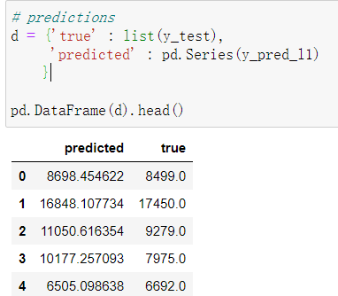
# predictions
d = {'true' : list(y_test),
     'predicted' : pd.Series(y_pred_l1)
    }

pd.DataFrame(d).head()