线性回归模型-最小二乘法Ordinary Least Squares

1.1 线性回归模型

下面是一系列的回归方法, 目标值是输入变量的线性组合, 定义$\hat{y}$表示要预测的值.
$\hat{y}(w,x)=w_0+w_1{x}_1+...+w_p{x}_p$
在这类模型中, 我们设向量$w=(w_1,...,w_p)$为coef_ (coefficient)并且 $w_0$为intercept_(bias).

1.1.1 最小二乘法(Ordinary Least Squares)

线性回归通过最小化观察值和线性模型的预测值之间的残差平方和来训练一组模型的参数$w=(w_1,...,w_p)$. 数学上需要解决如下问题:
$\underset{w}{\min }{\Vert Xw-y\Vert }_2^2$
LinearRegression 将会调用fit方法, 数据X, y并且把参数值w存在coef_中, $w_0$存在模型的intercept_中.

>>> from sklearn import linear_model
>>> reg = linear_model.LinearRegression()
>>> reg.fit([[0, 0], [1, 1], [2, 2]], [0, 1, 2])
...                                       
LinearRegression(copy_X=True, fit_intercept=True, n_jobs=None,
                 normalize=False)
>>> reg.coef_
array([0.5, 0.5])

然而, 最小二乘法的参数估计依赖模型特征之间的线性无关性. 当各特征之间存在相关性并且X的各列数据之间是线性相关时, X矩阵就会接近奇异值并且产生一个较大的方差, 最小二乘估计对收集观察数据时产生的随机误差十分敏感. 当收集数据是没有进行有针对性的设计避免随机误差, 将会产生多重共线性multicollinearity问题.

实例

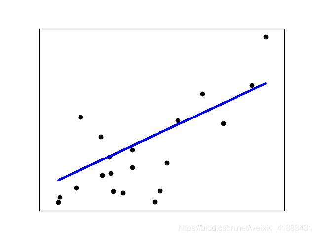
这一实例只使用一维数据集的第一个特征数据, 目的是在二维平面图中能够说明这一算法.图中的直线, 代表线性回归模型尝试画出一条直线, 这条线能够最小化所有观察值与预测值之间残差平方和, 其中观察值在数据集中, 预测值是线性模型预测出来的.

代码

  import matplotlib.pyplot as plt
  import numpy as np
  from sklearn import datasets, linear_model
  from sklearn.metrics import mean_squared_error, r2_score
 
  # Load the diabetes dataset
  diabetes = datasets.load_diabetes()
 
 print(type(diabetes.data))
 print(diabetes.data.shape)
 
 # Use only one feature
 diabetes_x = diabetes.data[:, np.newaxis, 2]
 
 print(type(diabetes_x))
 print(diabetes_x.shape)
 
 # Split the data into training/testing sets
 diabetes_x_train = diabetes_x[:-20]
 diabetes_x_test = diabetes_x[-20:]
 
 
 print(diabetes_x_train.shape)
 print(diabetes_x_test.shape)
 
 # Split the targets into training/testing sets
 diabetes_y_train = diabetes.target[:-20]
 diabetes_y_test = diabetes.target[-20:]
 
 # Create linear regression object
 regr = linear_model.LinearRegression()
 
 # Train the model using the training sets
 regr.fit(diabetes_x_train, diabetes_y_train)
 
 # Make predictions using the testing set
 diabetes_y_pred = regr.predict(diabetes_x_test)
 
 # The coefficients
 print('Coefficients: \n', regr.coef_)
 
 # The mean squared error
 print('Mean squared error: %.2f' % mean_squared_error(diabetes_y_test, diabetes_y_pred))
 
 # Explained variance score: 1 is perfect prediction
 print('Variance score: %.2f' % r2_score(diabetes_y_test, diabetes_y_pred))
 
 # Plot outputs
 plt.scatter(diabetes_x_test, diabetes_y_test, color = 'black')
 plt.plot(diabetes_x_test, diabetes_y_pred, color = 'blue', linewidth = 3)
 
 plt.xticks(())
 plt.yticks(())
 
 plt.show()

运行结果

n ordinary_least_squares.py 
<class 'numpy.ndarray'>
(442, 10)
<class 'numpy.ndarray'>
(442, 1)
(422, 1)
(20, 1)
Coefficients: 
 [938.23786125]
Intercept: 
 152.91886182616167
Mean squared error: 2548.07
Variance score: 0.47

知识

1. np.newaxis的使用
2. sklearn.metrics.r2_score