【学习笔记】Data Mining

---

Week1

Topic: Data Mining Intro & Data Preprocessing

---

1. Definition

Data mining is defined as the process of discovering patterns in data

• The process must be automatic or (more usually) semiautomatic.
• The patterns discovered must be meaningful in that they lead to some advantage.

2. Why

2.1 Descriptive

• Characterization and Discrimination
• The mining of frequent patterns, associations, and correlations

2.2 Predictive

• Classification and regression
• Clustering analysis：analyze class-labeled (training) data sets, clustering analyzes data objects without consulting class labels.
• Outlier analysis：a.k.a. anomaly mining

3. Process

1. Data cleaning：to remove noise and inconsistent data
2. Data integration：where multiple data sources may be combined
3. Data selection：where data relevant to the analysis task are retrieved from the database
4. Data transformation：where data are consolidated into forms appropriate
5. Data mining：extract data patterns
6. Pattern evaluation：to identify useful patterns based on interestingness measures
7. Knowledge presentation：where visualization and knowledge present

4. Input and Output

4.1 Input

• Concept: kinds of things that can be learned

1. Classification learning: predicting a discrete class
2. Association learning: detecting associations between features
3. Clustering: grouping similar instances into clusters
4. Numeric prediction: predicting a numeric quantity

• Instance: the individual, independent examples of a concept to be learned

1. Other names: tuple, case…

• Attributes: measuring aspects of an instance

1. Nominal
2. Ordinal
3. Interval
4. Ratio

4.2 Output: Knowledge representation

• Tables
• Linear models
• Trees
• Rules
• Classification rules：(if … then…) Alternative to decision trees, (e.g., if a<3, then b)
• Association rules：Classification rules + Support/Confidence

1. Support: number of instances predicted correctly
2. Confidence: number of correct predictions, as proportion of all instances that rule applies to

• Rules with exceptions：(if...then...Except...if...then...)Add exception condition
• Rules involving relations：Compare ('>' or '<') the relations, not specific number
• Instance-based representation：rote learning or lazy learning，e.g. KNN
• Clusters

5. Data Preprocessing

5.1 Why

5.1.1 How to measure Data Quality

• Accuracy: correct or wrong, accurate or not
• Completeness: not recorded, unavailable …
• Consistency: some modified but some not dangling …
• Timeliness: timely update?
• Believability: how trustable the data are correct?
• Interpretability: how easily the data can be understood?

5.2 How

• Data Cleaning：Fill in missing values, smooth noisy data, identify or remove outliers, and resolve inconsistencies
• Data Integration：Integration of multiple databases, data cube, or files
• Data Reduction：

1. Dimensionality reduction
2. Numerosity reduction
3. Data compression

• Data Transformation and Data Discretization

1. Normalization
2. Concept hierarchy generation

6. Data Cleaning

6.1 Issues with Real-World Data

• incomplete: lacking attribute values, lacking certain attributes of interest, or containing only aggregate data
• noisy: containing noise, errors, or outliers
• inconsistent: containing discrepancies in codes or names
• intentional (e.g., disguised missing data)

6.2 Noisy Data

Incorrect attribute values may be due to

• faulty data collection instruments
• data entry problems
• data transmission problems
• technology limitation
• inconsistency in naming convention

Other data problems which require data cleaning

• duplicate records
• incomplete data
• inconsistent data

6.3 How to handle noise

• Binning：first sort data and partition into (equal-frequency) bins ，then one can smooth by bin means, smooth by bin median, smooth by bin boundaries, etc.

• Regression：smooth by fitting the data into regression functions
• Clustering：detect and remove outliers
• Combined computer and human inspection

7. Data integration

7.1 Why

• Schema integration：Integrate metadata from different sources（e.g., A.cust-id = B.cust-# = C.customer_id）
• Entity identification problem：Identify real world entities from multiple data sources, e.g., Bill Clinton = William Clinton
• Detecting and resolving data value conflicts：For the same real-world entity, attribute values from different sources are different，e.g., metric vs. British units

7.2 How

• Correlation Analysis (Nominal Data)：X2 (chi-square) test 卡方检验
• Correlation Analysis (Numeric Data)：correlation coefficient (Pearson’s product moment coefficient)(-1 to 1) 皮尔逊系数
• Covariance (Numeric Data)：协方差

8. Data Reduction

• Wavelet Transform
• Principal Component Analysis (PCA)
• Attribute Subset Selection - Heuristic Search
• Attribute Creation：1. Attribute extraction，2. Mapping data to new space，3. Attribute construction
• Numerosity Reduction：1. Parametric methods (e.g., regression)，2. Non-parametric methods（histograms, clustering, sampling...）

1. Parametric data reduction:  Linear regression，Multiple regression，Log-linear model
2. Histogram Analysis： Divide data into buckets and store average (sum) for each bucket
3. Clustering：Partition data set into clusters based on similarity, and store cluster representation
4. Sampling：Choose a representative subset of the data（e.g., 1. Simple random sampling，2. Cluster Sampling，3. Stratified sampling）

• Data Compression：String compression，Audio/video compression，Time sequence

9. Data Transformation

9.1 Definition

A function that maps the entire set of values of a given attribute to a new set of replacement values. each old value can be identified with one of the new values

9.2 Methods

• Smoothing: Remove noise from data
• Attribute construction - New attributes constructed from the given ones (e.g.: PCA)
• Aggregation: Summarization
• Normalization: Scaled to fall within a smaller, specified range (e.g: -1 to 1) , including min-max; z-score: normalization by decimal scaling
• Discretization: Concept hierarchy climbing

9.3 Data Discretization Methods

9.3.1 Typical methods

All the methods can be applied recursively

• Binning:  Top-down split, unsupervised
• Histogram analysis: Top-down split, unsupervised
• Clustering analysis (unsupervised, top-down split or bottom-up merge)
• Decision-tree analysis (supervised, top-down split)
• Correlation (e.g., X2) analysis (unsupervised, bottom-up merge)

9.3.2 Simple Discretization : Bining

• Equal-width (distance) partitioning
• Equal-depth (frequency) partitioning

9.4 Concept Hierarchy Generation

• Specification of a partial/total ordering of agributes at the schema level by users or experts：e.g., street < city < state < country
• Specification of a hierarchy for a set of values by explicit data grouping：e.g.,{Nanjing, Suzhou}＜JiangSu
• Specification of only a partial set of agributes：E.g., only street < city, not others
• Automatic generation of hierarchies (or agribute levels) by the analysis of the number of distinct values：E.g., for a set of ajributes: {street, city, state, country}

---

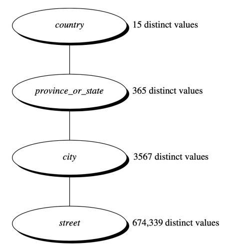
Week2

Topic: Data Warehousing and OLAP & Classification

---

1. Data Warehouse Concepts

• A decision support database that is maintained separately from the organization‘s operational database.
• Support information processing by providing a solid platform of consolidated, historical data for analysis.
• A data warehouse is a subject-oriented, integrated, time-variant, and nonvolatile collection of data in support of management‘s decisionmaking process

2. Why

2.1 High performance for both systems

• DBMS: tuned for Online Transaction processor (OLTP): access methods, indexing, concurrency control, recovery
• Warehouse: tuned for OLAP: complex OLAP queries, multidimensional view, consolidation

2.2 Different functions and different data

• missing data: Decision support requires historical data which operational Bs do not typically maintain
• data consolidation: Decision support requires consolidation of data from heterogeneous sources
• data quality: different sources typically use inconsistent data representations, codes and formats which have to be reconciled

3. OLTP vs. OLAP

4. Data Warehouse Architecture

4.1 Extraction, Transformation, and Loading (ETL)

• Data extraction：get data from multiple, heterogeneous, and external sources
• Data cleaning：detect errors in the data and rectify them when possible
• Data transformation：convert data from legacy or host format to warehouse format
• Load：sort, summarize, consolidate, compute views, check integrity, and build indices and partitions
• Refresh：propagate the updates from the data sources

4.2 Metadata Repository

Meta data is the data defining warehouse objects. It stores:

• Description of the structure of the data warehouse：schema, view, dimensions, hierarchies, derived data defn, data mart locations and contents
• Operational meta-data：data lineage (history of migrated data and transformation path), currency of data (active, archived, or purged), monitoring information (warehouse usage statistics, error reports, audit trails)
• The algorithms used for summarization
• The mapping from operational environment to the data warehouse
• Data related to system performance：warehouse schema, view and derived data definitions
• Business data：business terms and definitions, ownership of data, charging policies

4.3 Three Data Warehouse Models

1. Enterprise warehouse：collects all of the information about subjects spanning the entire organization
2. Data Mart：a subset of corporate-wide data that is of value to a specific groups of users. Its scope is confined to specific, selected groups, such as marketing data mart
3. Virtual warehouse：A set of views over operational databases，Only some possible summary views may be materialized

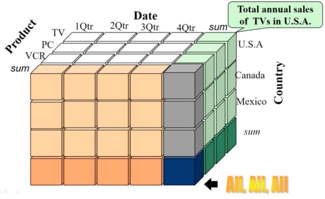
5. Data Cube

From Tables and Spreadsheets to Data Cubes

• A data warehouse is based on a multidimensional data model which views data in the form of a data cube
• A data cube, such as sales, allows data to be modelled and viewed in multiple dimensions

1. Dimension tables, such as item (item_name, brand, type), or time (day, week, month, quarter, year)
2. Fact table contains measures (such as dollars sold) and keys to each of the related dimension tables

• In data warehousing literature, an n-D base cube is called a base cuboid. The top most 0-D cuboid, which holds the highest-level of summarization, is called the apex cuboid. The lattice of cuboids forms a data cube.

3-D Data Cube：
referred to as a cuboid Cube: A lattice of Cuboids

5.1 Conceptual Modeling of Data Warehouses

Modelling data warehouses: dimensions & measures

• Star schema: A fact table in the middle connected to a set of dimension tables
• Snowflake schema: A refinement of star schema where some dimensional hierarchy is normalized into a set of smaller dimension tables, forming a shape similar to snowflake
• Fact constellations: Multiple fact tables share dimension tables, viewed as a collection of stars, therefore called galaxy schema or fact constellation

Star schema Snowflake schema Fact constellations

5.2 Data Cube Measures 

• A multidimensional point in the data cube space can be defined by a set of dimension – value pairs. For example, 〈time = “Q1”, location = “Vancouver”, item = “computer”〉
• A data cube measure is a numeric function that can be evaluated at each point in the data cube space.
• A measure value is computed for a given point by aggregating the data corresponding to the respective dimension

Three Categories:

1. Distributive: if the result derived by applying the function to n aggregate values is the same as that derived by applying the function on all the data without partitioning
   E.g., count(), sum(), min(), max()
    
2. Algebraic: if it can be computed by an algebraic function with M arguments (where M is a bounded integer), each of which is obtained by applying a distributive aggregate function
   E.g., avg(), standard_deviation()
    
3. Holistic: if there is no constant bound on the storage size needed to describe a sub aggregate.
   E.g., median(), mode(), rank()

Example

6. Typical OLAP Operations

• Roll up (drill-up)：summarize data by Climbing up hierarchy or by dimension reduction
• Drill down (roll down)：reverse of roll-up
• Slice and dice：project and select
• Pivot (rotate)：reorient the cube, visualization 3D to series of 2D planes
• drill across：involving (across) more than one fact table
• drill through：through the bottom level of the cube to its back-end relational tables (using SQL)

7. Design of Data Warehouse：A Business Analysis Framework

Four views regarding the design of a data warehouse：

• Top-down view - allows selection of the relevant information necessary for the data warehouse
• Data source view - exposes the information being captured, stored, and managed by operational systems
• Data warehouse view - consists of fact tables and dimension tables
• Business query view - sees the perspectives of data in the warehouse from the view of end-user

7.1 Data Warehouse Design Process

• Top-down, bottom-up approaches or a combination of both

1. Top-down: Starts with overall design and planning (mature)
2. Bottom-up: Starts with experiments and prototypes (rapid)

• From software engineering point of view

1. Waterfall: structured and systematic analysis at each step before proceeding to the next
2. Spiral: rapid generation of increasingly functional systems, short turn around time, quick turn around

Typical data warehouse design process：

1. Choose a business process to model (e.g., orders, invoices, etc.)
2. Choose the grain (atomic level of data) of the business process (e.g., individual transactions, individual daily snapshots, and so on)
3. Choose the dimensions that will apply to each fact table record
4. Choose the measure that will populate each fact table record

7.2 Data Warehouse Usage

• Information processing：supports querying, basic statistical analysis, and reporting using crosstabs, tables, charts and graph
• Analytical processing：supports basic OLAP operations, slice-dice, drilling, pivoting
• Data mining：supports associations, constructing analytical models, performing classification and prediction, and presenting the mining results using visualization tools

7.3 Online Analytical Mining (OLAM)

• High quality of data in data warehouses：DW contains integrated, consistent, cleaned data
• Available information processing structure surrounding data warehouses：Web accessing, service facilities, reporting and OLAP tools
• OLAP-based exploratory data analysis：Mining with drilling, dicing, pivoting, etc
• Online selection of data mining functions：Integration and swapping of multiple mining functions, algorithms, and tasks

8. Data Warehouse Implementation

8.1 The “Compute Cube” Operator

Transform it into SQL-Like language

SELECT item, city, year, SUM (amount)
FROM SALES
CUBE BY item, city, year

8.2 Indexing OLAP Data: Bitmap Index and Join Index

8.2.1 Bitmap Index

 8.2.2 Join Index

In data warehouses, join index relates the values of the dimensions of a start schema to rows in the fact table.

8.3 OLAP Server Architectures

• Relational OLAP (ROLAP)

1. Use relational or extended-relational DBMS to store and manage warehouse data and OLAP middle ware
2. Include optimization of DBMS backend, implementation of aggregation navigation logic, and additional tools and services
3. Greater scalability

• Multidimensional OLAP (MOLAP)

1. Sparse array-based multidimensional storage engine
2. Fast indexing to pre-computed summarized data

• Hybrid OLAP (HOLAP) (e.g., Microsoft SQLServer)

1. Flexibility, e.g., low level: relational, high-level: array

• Specialized SQL servers (e.g., Redbricks)

1. Specialized support for SQL queries over star/snowflake schemas

9. Data Generalization by Attribute-Oriented Induction

9.1 Example of AOI

Describe general characteristics of graduate students in the University database (given the attributes name, gender, major, birth place, birth date, residence, phone# (telephone number), and gpa (grade point average).

Step 1. Fetch relevant set of data using an SQL statement, e.g.,

Select * (i.e., name, gender, major, birth_place, birth_date, residence, phone#, gpa)
from student
where student status in ("Msc", "MBA", "PhD" }

Step 2. Perform attribute-oriented induction（AOI）

Step 3. Present results in generalized relation, cross-tab, or rule forms

9.2 Basic Principles of AOI

• Data focusing: task-relevant data, including dimensions, and the result is the initial relation
• Attribute-removal: remove attribute A if there is a large set of distinct values for A but (1) there is no generalization operator on A, or (2) A‘s higher level concepts are expressed in terms of other attributes
• Attribute-generalization: If there is a large set of distinct values for A, and there exists a set of generalization operators on A, then select an operator and generalize A
• Attribute-threshold control: typical 2-8, specified/default
• Generalized relation threshold control: control the final relation/rule size

9.3 AOI: Basic Algorithms

1. InitialRel: Query processing of task-relevant data, deriving the initial relation.
2. PreGen: Based on the analysis of the number of distinct values in each attribute, determine generalization plan for each attribute: removal? or how high to generalize?
3. PrimeGen: Based on the PreGen plan, perform generalization to the right level to derive a “prime generalized relation", accumulating the counts.
4. Presentation: User interaction: (1) adjust levels by drilling, (2) pivoting, (3) mapping into rules, cross tabulations, visualization presentations.

9.4 AOI vs. Cube-Based PLAP

Similarity:

• Data generalization
• Presentation of data summarization at multiple levels of abstraction
• Interactive drilling, pivoting, slicing and dicing

Differences:

• OLAP has systematic preprocessing, query independent, and can drill down to rather low level OLAP
• AOI has automated desired level allocation, and may perform dimension relevance analysis/ranking when there are many relevant dimensions
• AOI works on the data which are not in relational forms

10. Classification: A two-step process

1. Model construction (Learning): describing a set of predetermined classes
2. Model usage (Classification): for classifying future or unknown objects

11. More contents: I passed here

• Decision Tree Induction
• Bayes Classification Methods
• Rule-Based Classification
• Model Evaluation and Selection
• Techniques to Improve Classification Accuracy: Ensemble Methods

---

Week3

Topic: Clustering & Prediction & Mining patterns, association and correlations

---

1. Cluster Analysis

• Finding similarities between data according to the characteristics found in the data and grouping similar data objects into clusters
• Unsupervised learning: no predefined classes (i.e. learning by observations vs. learning by examples: supervised)

The quality of a clustering method depends on：

1. the similarity measure used by the method
2. its implementation
3. Its ability to discover some or all of the hidden patterns

2. Measure the Quality of Clustering

Dissimilarity/Similarity metric

• Similarity is expressed in terms of a distance function, typically metric: d(i, j)
• The definitions of distance functions are usually rather different for intervalscaled, boolean, categorical, ordinal ratio, and vector variables
• Weights should be associated with different variables based on applications and data semantics

3. Considerations for Cluster Analysis

• Partitioning criteria：Single level vs. hierarchical partitioning (often, multi-level hierarchical partitioning is desirable)
• Separation of clusters：Exclusive (e.g., one customer belongs to only one region) vs. non-exclusive (e.g., one document may belong to more than one class)
• Similarity measure：Distance-based (e.g., Euclidian, road network, vector) vs. connectivity-based (e.g., density or contiguity)
• Clustering space：Full space (often when low dimensional) vs. subspaces (often in high-dimensional clustering)

4. Major Clustering Approaches（*）

• Partitioning approach：Construct various partitions and then evaluate them by some criterion, e.g., minimizing the sum of square errors
  Typical methods: k-means, k-medoids, CLARANS
• Hierarchical approach：Create a hierarchical decomposition of the set of data (or objects) using some criterion
  Typical methods: Diana, Agnes, BIRCH, CAMELEON
• Density-based approach：Based on connectivity and density functions
  Typical methods: DBSCAN, OPTICS, DenClue
• Grid-based approach：based on a multiple-level granularity structure
  Typical methods: STING, WaveCluster, CLIQUE
• Model-based：A model is hypothesized for each of the clusters and tries to find the best fit of that model to each other
  Typical methods: EM, SOM, COBWEB
• Frequent pattern-based：Based on the analysis of frequent patterns
  Typical methods: p-Cluster
• User-quided or constraint-based：Clustering by considering user-specified or application-specific constraints
  Typical methods: COD (obstacles), constrained clustering
• Link-based clustering：Objects are often linked together in various ways
  Massive links can be used to cluster objects: SimRank, LinkClus

5. Partitioning method

• Partitioning a database D of n objects into a set of k clusters, such that the sum of squared distances is minimized (where ci is the centroid or medoid of cluster Ci , p means other points)
• Given k, find a partition of k clusters that optimizes the chosen partitioning criterion

1. Global optimal: exhaustively enumerate all partitions (NP hard)
2. Heuristic methods: k-means and k-medoids algorithms

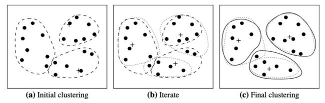
5.1 K-Means

The k-means algorithm defines the centroid of a cluster as the mean value of the points within the cluster.

Given k, the k-means algorithm is implemented in four steps:

1. Randomly selects k of the objects in D
2. Compute “seed points” as the centroids of the clusters of the current partitioning (the centroid is the center, i.e., mean point, of the cluster)
3. Assign each object to the cluster with the nearest seed point
4. Go back to Step 2, stop when the assignment does not change

 Limits:

• The k-means method is not guaranteed to converge to the global optimum and often terminates at a local optimum. The results may depend on the initial random selection of cluster centers.
• The time complexity of the k-means algorithm is O(nkt), where n is the total number of objects, k is the number of clusters, and t is the number of iterations. Normally, k ≪ n and t ≪ n. Therefore, the method is relatively scalable and efficient in processing large data sets.
• Sensitive to noise and outliers: a small number of such data can substantially influence the mean value

5.2 K-Medoids

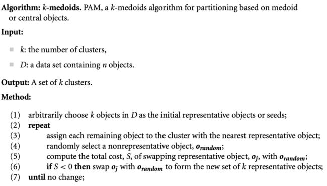
Improvements：

• CLARA: Instead of taking the whole data set into consideration, CLARA uses a random sample of the data set. The PAM algorithm is then applied to compute the best medoids from the sample. Ideally, the sample should closely represent the original data set. In many cases, a large sample works well if it is created so that each object has equal probability of being selected into the sample.
• CLARANS: First, it randomly selects k objects in the data set as the current medoids. It then randomly selects a current medoid x and an object y that is not one of the current medoids. Can replacing x by y improve the absolute error criterion? If yes, the replacement is made. The set of the current medoids after the l steps is considered a local optimum. CLARANS repeats this randomized process m times and returns the best local optimal as the final result.

6. Hierarchical Methods

Use distance matrix as clustering criteria. This method does not require the number of clusters k as an input, but needs a termination condition.

6.1 AGNES

This is a single-linkage approach in that each cluster is represented by all the objects in the cluster, and the similarity between two clusters is measured by the similarity of the closest pair of data points belonging to different clusters.

The cluster-merging process repeats until all the objects are eventually merged to form one cluster.

6.2 DIANA

• All the objects are used to form one initial cluster.
• The cluster is split according to some principle such as the maximum Euclidean distance between the closest neighboring objects in the cluster.
• The cluster-splitting process repeats until, eventually, each new cluster contains only a single object.

6.3 Dengorgram

A tree structure called a dendrogram is commonly used to represent the process of hierarchical clustering. It shows how objects are grouped together (in an agglomerative method) or partitioned (in a divisive method) step-by-step.

 6.4 Example

Key Problem: When shall we stop

Four widely used measures for distance between clusters are as follows, where |p − pʹ| is the distance between two objects or points, p and pʹ; mi is the mean for cluster, Ci; and ni is the number of objects in Ci. They are also known as linkage measures.

Distance between Clusters

Example: 

 Original Data Samples

before - distance matrix after - average

 ... till last one cluster

Improvement

• BIRCH
• CHAMELEOM

6.5 Balanced Iterative Reducing and Clustering using Hierarchies (BIRCH)

BIRCH uses the notions of clustering feature to summarize a cluster, and clustering feature tree (CF-tree) to represent a cluster hierarchy.

• Phase 1: scan DB to build an initial in-memory CF tree (a multi-level compression of the data that tries to preserve the inherent clustering structure of the data)
• Phase 2: BIRCH applies a (selected) clustering algorithm to cluster the leaf nodes of the CF-tree, which removes sparse clusters as outliers and groups dense clusters into larger ones.

6.5.1 clustering feature (CF)

Consider a cluster of n d-dimensional data objects or points. The clustering feature (CF) of the cluster is a 3-D vector summarizing information about clusters of objects. where LS is the linear sum of the n points and SS is the square sum of the data points

Example

6.5.2 CF-tree

CF-tree has two parameters: branching factor, B, and threshold, T

• The branching factor specifies the maximum number of children per nonleaf node.
• The threshold parameter specifies the maximum diameter of subclusters stored at the leaf nodes of the tree.

6.5.3 Steps of BIRCH

For each point in the input：

1. Find closest leaf entry
2. Add point to leaf entry and update CF
3. If entry diameter > max_diameter, then split leaf, and possibly parents

Algorithm is O(n)

6.5.4 Concerns

• Sensitive to insertion order of data points
• Since we fix the size of leaf nodes, so clusters may not be so natural
• Clusters tend to be spherical given the radius and diameter measures

总结一下BIRCH算法的主要优缺点。它的优点是聚类速度快，可以识别噪音点，还可以对数据集进行初步分类的预处理；主要缺点有：对高维特征数据、非凸数据集效果不好；由于CF个数的限制会导致与真实类别分布不同.

6.6 Chameleon: Multiphase Hierarchical Clustering Using Dynamic Modeling

• Chameleon is a hierarchical clustering algorithm that uses dynamic modeling to determine the similarity between pairs of clusters.
• Chameleon: K-NN based
• Chameleon uses a graph partitioning algorithm to partition the k-nearest- neighbor graph into a large number of relatively small subclusters

7. ​​​​​​​Density-Based Clustering Methods

Two parameters:

• Eps (ε): Maximum radius of the neighbourhood
• MinPts: Minimum number of points in an Eps-neighbourhood of that point

7.1 DBSCAN: Density-Based Clustering Based on Connected Regions with High Density

• Arbitrary select a point p
• Check whether the eps of p contains at least MinPts objects. If not, p is marked as a noise point.
• Otherwise, a new cluster C is created for p, and all the objects in the eps of p are added to a candidate set, N
• iteratively add objects in N to the same cluster. For an object pʹ in N, if the eps of pʹ has at least MinPts objects, those objects in the eps of pʹ are also added to N. (density- reachable)
• Stop when N is empty
• Continue the process until all points has been processed

8. Grid-Based Method​​​​​​​

a grid-based clustering method takes a space-driven approach by partitioning the embedding space into cells independent of the distribution of the input objects.

Two Examples:

• STING:explores statistical information stored in the grid cells
• CLIQUE: represents a grid- and density-based approach for subspace clustering in a high-dimensional data space.

8.1 STING

STING is a grid-based mulIresoluIon clustering technique in which the embedding spaIal area of the input objects is divided into rectangular cells.

• Each cell at a high level is partitioned to form a number of cells at the next lower level.
• Statistical information regarding the attributes in each grid cell is precomputed and stored as statistical parameters.
• The statistical parameters of higher-level cells can easily be computed from the parameters of the lower-level cells.
• Use a top-down approach to answer spatial data queries
• Start from a pre-selected layer-typically with a small number of cells 
• For each cell in the current level compute the confidence interval

Advantages:

• Query-independent, easy to parallelize, incremental update
• O(K), where K is the number of grid cells at the lowest level

Disadvantages:

• All the cluster boundaries are either horizontal or vertical, and no diagonal boundary is

8.2 CLIQUE (Clustering In QUEst)

CLIQUE (CLustering In QUEst) is a simple grid-based method for finding density- based clusters in subspaces.

Two Steps:

1. In the first step, CLIQUE partitions the d-dimensional data space into nonoverlapping rectangular units, identifying the dense units among these. CLIQUE finds dense cells in all of the subspaces.
2. In the second step, CLIQUE uses the dense cells in each subspace to assemble clusters, which can be of arbitrary shape.

9. Evaluation of Clustering

9.1 Determine the Number of Clusters

• Simple Method: set the number of clusters to about √n/2 for a data set of n points.
• Elbow method：Use the turning point in the curve of sum of within cluster variance w.r.t the # of clusters

我们知道k-means是以最小化样本与质点平方误差作为目标函数，将每个簇的质点与簇内样本点的平方距离误差和称为畸变程度(distortions)，那么，对于一个簇，它的畸变程度越低，代表簇内成员越紧密，畸变程度越高，代表簇内结构越松散。 畸变程度会随着类别的增加而降低，但对于有一定区分度的数据，在达到某个临界点时畸变程度会得到极大改善，之后缓慢下降，这个临界点就可以考虑为聚类性能较好的点。

• Cross Validation

9.2 Clustering Quality

• extrinsic methods：Compare the clustering against the ground truth and measure
• intrinsic methods：evaluate the goodness of a clustering by considering how well the clusters are separated.

10. More Prediction

• Numeric Prediction
• Linear Regression

1. ​​​​​​​​​​​​​​Linear Regression
2. Non-Linear Regression
3. Classification by regression

• Logistic Regression

1. ​​​​​​​​​​​​​​Logit transformation

• Support Vector Machines

1. ​​​​​​​​​​​​​​Margin and support vectors

2. Linear Separable
3. Linear Inseparable

11. Data mining tasks

• Association, correlation, and causality analysis
• Sequential, structural (e.g., sub-graph) patterns
• Pattern analysis in spatiotemporal, multimedia, time-series, and stream data
• Classification: discriminative, frequent pattern analysis
• Cluster analysis: frequent pattern-based clustering
• Data warehousing: iceberg cube and cube-gradient
• Semantic data compression: fascicles
• Broad applications

12. Frequent Patterns

• itemset: A set of one or more items
• k-itemset X= {x1,..., xk}: An itemset that contains k items
• (absolute) support, or, support count of X: Frequency or occurrence of an itemset X (3)
• (relative) support, s, is the fraction of transactions that contains X (i.e., the probability that a transaction contains X) (0.6)
• An itemset X is frequent if X‘s relative support is no less than a minimum support threshold

13. Association Rules

Find all the rules X --> Y with minimum support and confidence

• support, s, probability that a transaction contains X ∪ Y
• confidence, c, the conditional probability of transactions in D containing X that also contain Y ( P(Y|B) ) .

Example：

14. Closed Patterns and Max-itemsets

• An itemset X is closed in a data set D if there exists no proper superitemset Y such that Y has the same support count as X in D 
• An itemset X is a maximal frequent itemset (or max-itemset) in a data set D if X is frequent, and there exists no super-itemset Y such that X ⊂Y and Y is frequent in D.
• Closed pattern is a lossless compression of freq. patterns

Example

15. Frequent Itemset Mining Method

• Apriori • Fggrowth • Closet

15.1 Apriori: Finding Frequent Itemsets by Confined Candidate Generation

• Apriori property: All nonempty subsets of a frequent itemset must also be frequent.
• Apriori Pruning principle (antimonotonicity): if a set cannot pass a test (infrequent), all of its supersets will fail the same test as well

Steps:

1. Initially, scan DB once to get frequent 1-itemset
2. self-joining: Generate length (k+1) candidate itemsets from length k frequent itemsets
3. Pruning: Test the candidates against DB
4. Terminate when no frequent or candidate set can be generated

Aprior example: min sup.=2 in this case

Improving Apriori:

• Scan Database only twice：Any itemset that is potentially frequent in DB must be frequent in at least one of the partitions of DB
• Reduce the Number of Candidates
• Sampling for Frequent Patterns

15.2 FP-growth: A Pattern-Growth Approach for Mining Frequent Itemsets

• Depth-first search
• Grow long patterns from short ones using local frequent items only

Example

Steps:

1. Scan DB once, find frequent 1-itemset
2. Sort frequent items in frequency descending order, f-list
3. Scan DB again, construct FP-tree
4. Starting at the frequent item header table in the FP-tree
5. Traverse the FP-tree by following the link of each frequent item p
6. Accumulate all of transformed prefix paths of item p to form p’s conditional pattern base

f-list and FP-tree

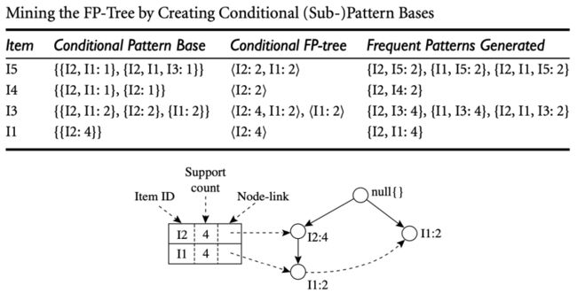conditional pattern base

• Completeness：Preserve complete information for frequent pattern mining
• Compactness：Items in frequency descending order， the more frequently occurring, the more likely to be shared

15.3 Mining Closed and Max PatternsL: CLOSET

• Flist: list of all frequent items in support ascending order
• Divide search space：Patterns having d but no a, etc.
• Find frequent closed pattern recursively

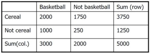
16. Correlation Rules

A correlation rule is measured not only by its support and confidence but also by the correlation between itemsets A and B

Lift can be used as a simple correlation measure (higher)

16.1 Correlation Rules: Lift 提升度

​​​​​​​

当lift>1，说明A和B之间有正相关关系，且数值越大正相关程度越高
当lift<1，说明A和B之间有负相关关系，且数值越小负相关程度越高（lift定义大于等于零）
当lift=1，说明A和B之间没有相关关系
 

---

Week4

Topic: 
Mining Complex Data types & Advanced & Data Mining Trends and Research Frontiers

---

1. Different data types

2. Mining Time Series Data

Methods for time series analyses

• Frequency-domain methods: Model-free analyses, well-suited to exploratory investigations - spectral analysis vs. wavelet analysis
• Time-domain methods: Auto-correlation and cross-correlation analysis
• Motif-based time-series analysis

2.1 Regression Analysis

• Linear and multiple regression
• Non-linear regression
• Generalized linear model, Poisson regression, log-linear models
• Regression trees：proposed in CART system
• Model tree: Each leaf holds a regression model—a multivariate linear equation for the predicted attribute

2.2 Trend Analysis

Categories of Time-Series Movements：

• Long-term or trend movements (Trend Curve) (T): general direction in which a time series is moving over a long interval of time
• Cyclic movements or cycle variations (C): long term oscillations about a trend line or curve - e.g., business cycles, may or may not be periodic
• Seasonal movements or seasonal variations (S) - i.e, almost identical patterns that a time series appears to follow during corresponding months of successive years.
• Irregular or random movements (I)

2.3 Similarity Search in Time Series Data

• Whole matching: find a sequence that is similar to the query sequence
• Subsequence matching: find all pairs of similar subsequences

2.3.1 discrete Fourier transform (DFT)

The Euclidean distance between two signals in the time domain is the same as their distance in the frequency domain （Parseval’s Theorem​​​​​​​）帕塞瓦尔定理

2.3.2 discrete wavelet transform (DWT)

2.4 Motif-Based Search and Mining in Time Series Data  模体

motif： A previously unknown, frequently occurring sequential pattern

2.4.1 SAX: Symbolic Aggregate approXimation

时间序列符号聚合近似方法

• Essentially an alphabet over the Piecewise Aggregate Approximation (PAA) rank
• Experiments show this approach is fast and simple, and has comparable search quality to that of DFT, DWT, and other dimensionality reduction methods.

Parameters: alphabet size, word (segment) length (or output rate)

1. Select probability distribution for TS
2. z-score Normalize TS
3. PAA: Within each time interval, calculate aggregated value (mean) of the segment
4. Partition TS range by equal-area partitioning
5. Label each segment with a_rank ∈∑ for aggregate’s corresponding partition rank

 SAX特性：

1. 可以进行数据降维。
2. 可以在符号表示上定义距离度量，并且满足下界定理。
3. 可以进行数据压缩。
4. SAX保留了原始时间序列的大体形状。SAX是一种符号表示法，因此字母表可以存储为位（bits）而不是双精度浮点数，从而节省了大量空间。

3. Mining Graphs and Networks

• graph (G.) definition: set of nodes joined by a set of lines (undirected graphs) or arrows (directed graphs)
• vertices: represent objects of interest connected with edge
• edges: represented by arcs connecting vertices;

3.1 Networks

• Graph Pattern Mining: Frequent subgraph patterns, closed graph patterns, Span vs. CloseGraph
• Statistical Modeling of Networks: Small world phenomenon, power law (log-tail) distribution, densification
• Clustering and Classification of Graphs and Homogeneous Networks
• Clustering, Ranking and Classification of Heterogeneous Networks
• Role Discovery and Link Prediction in Information Networks: PathPredict
• Similarity Search and OLAP in Information Networks: PathSim, GraphCube
• Evolution of Social and Information Networks: EvoNetClus

 4. Advanced Pattern Mining

4.1 Mining in Multilevel Association Rule

• Flexible min-support thresholds: Some items are more valuable but less frequent
• Redundancy Filtering: Some rules may be redundant due to "ancestor" relationships between items
• A rule is redundant if its support is close to the “expected” value, based on the rule's ancestor

4.2 Mining Multidimensional Association

• Categorical Attributes: finite number of possible values, no ordering among values ---- data cube approach 
• Quantitative Attributes: Numeric, implicit ordering among values ---- discretization, clustering, and gradient approaches

4.3 Negative and Rare Patterns

• Rare patterns: Very low support but interesting
• Negatively correlated patterns that are infrequent tend to be more interesting than those that are frequent

• Null transaction ¬A∩¬B
• Null Invariance的意思是，值不随着null-transactions的改变而改变。

5. Advanced Classification Methods

• Classification by Backpropagation：Neural Network
• Lazy Learners：Instance-Based Methods
• Instance-Based Methods： Store training examples and delay the processing (“lazy evaluation‘) until a new instance must be classified

Typical approaches of Lazy Learners:

• k-nearest neighbor approach
• Locally weighted regression
• Case-based reasoning (CBR)

7. Other Methodologies of Data Mining

7.1 Statistical Data Mining

• Factor analysis：determine which variables are combined to generate a given factor
• Discriminant analysis：predict a categorical response variable, commonly used in social science
• Time Series
• Quality Control：displays group summary charts
• Survival Analysis：predicts the probability that a patient undergoing a medical treatment would survive at least to time t (life span prediction)

7.2 Data Mining Result Visualisation

• Scatter plots and boxplots (obtained from descriptive data mining)
• Decision trees
• Association rules
• Clusters
• Outliers
• Generalized rules

8. Privacy, Security and Social Impacts of Data Mining

The real privacy concern: unconstrained access of individual records, especially privacy-sensitive information

• Method 1: Removing sensitive IDs associated with the data
• Method 2: Data security-enhancing methods
  Multi-level security model: permit to access to only authorized level
  Encryption: e.g., blind signatures, biometric encryption, and anonymous databases (personal information is encrypted and stored at different locations)
• Method 3: Privacy-preserving data mining methods

---

Week5

Topic: Introduction to Data Mining: NLP

---

1. Applications of NLP

• Automate routine tasks: Chatbots powered by NLP can process a large number of routine tasks that are handled by human agents today, freeing up employees to work on more challenging and interesting tasks.
• Improve search: NLP can improve on keyword matching search for document and FAQ retrieval by disambiguating word senses based on context (for example, “carrier” means something different in biomedical and industrial contexts), matching synonyms (for example, retrieving documents mentioning “car” given a search for “automobile”), and taking morphological variation into account (which is important for non-English queries). Effective NLP-powered academic search systems can dramatically improve access to relevant cuttingedge research for doctors, lawyers, and other specialists.
• Search engine optimization: NLP is a great tool for getting your business ranked higher in online search by analyzing searches to optimize your content.Analyzing and organizing large document collections: NLP techniques such as document clustering and topic modeling simplify the task of understanding the diversity of content in large document collections, such as corporate reports, news articles, or scientific documents. These techniques are often used in legal discovery purposes.
• Social media analytics: NLP can analyze customer reviews and social media comments to make better sense of huge volumes of information. Sentiment analysis identifies positive and negative comments in a stream of social-media comments, providing a direct measure of customer sentiment in real time.
• Market insights: With NLP working to analyze the language of your business’ customers, you’ll have a better handle on what they want, and also a better idea of how to communicate with them. Aspect-oriented sentiment analysis detects the sentiment associated with specific aspects or products in social media (for example, “the keyboard is great, but the screen is too dim”), providing directly actionable information for product design and marketing. 
• Moderating content: If your business attracts large amounts of user or customer comments, NLP enables you to moderate what’s being said in order to maintain quality and civility by analyzing not only the words, but also the tone and intent of comments

2. Bag Of Words

Bag-of-words models treat documents as unordered collections of tokens or words (a bag is like a set, except that it tracks the number of times each element appears).

Bag-of-words models are often used for efficiency reasons on large information retrieval tasks such as search engines. They can produce close to state-of-the-art results with longer documents.

Nevertheless, it suffers from some shortcomings, such as：

• Vocabulary: The vocabulary requires careful design, most specifically in order to manage the size, which impacts the sparsity of the document representations.
• Sparsity: Sparse representations are harder to model both for computational reasons (space and time complexity) and also for information reasons, where the challenge is for the models to harness so little information in such a large representational space.
• Meaning: Discarding word order ignores the context, and in turn meaning of words in the document (semantics). Context and meaning can offer a lot to the model, that if modeled could tell the difference between the same words differently arranged (“this is interesting” vs “is this interesting”), synonyms (“old bike” vs “used bike”), and much more.

3. NLP Preprocessing

• Tokenization
• Stop word removal
• Stemming and lemmatization 词干提取和词形还原

4. Term Frequency-Inverse Document Frequency （TF-IDF）

5. Topic Modelling

• Latent Semantic Analysis (LSA)
• Latent Dirichlet Allocation (LDA)

6. Word Embedding

• Word2vec
• GloVe (Global Vectors for Word Representation)

7. Sentiment analysis

• Aspect-based sentiment analysis （ABSA）
• 细粒度情感分析(fine-grained SA)

拓展阅读

聚类算法（BIRCH）_整得咔咔响的博客-CSDN博客

---

课程版权©限制，禁止搬运（大概）