PyTorch深度学习-03梯度下降（快速入门）

---

1.Gradient Descent (梯度下降)

1.1 Optimization Problem (优化问题)

找使目标函数最小的权重（求函数最小值）

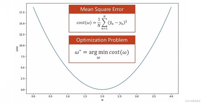
1.2 Gradient Descent algorithm (梯度下降算法)

确定初始权重需要往左移还是往右移才能得到目标权重

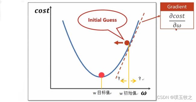
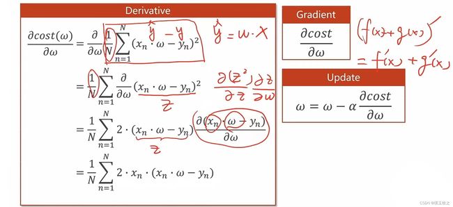
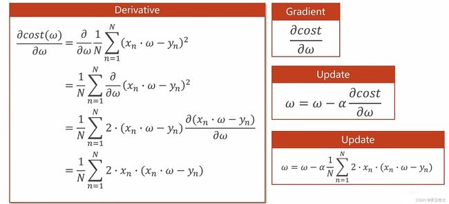
1.2.1 Gradient (梯度)

用目标函数对权重求导，就可以得到它的上升方向。负导数为下降方向。

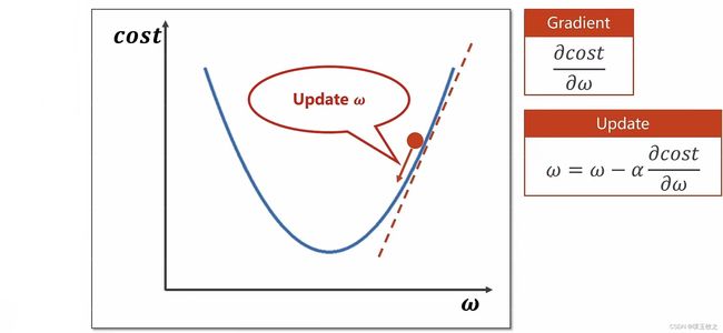
1.2.2 Update (更新权重)

权重减学习率乘导数

• 学习率 (步长)：表示往前移动多远 (通常学习率取值较小)
  

• 贪心算法：每次迭代都朝着下降最快的方向走一步，梯度下降不一定能得到最优结果，但能得到在局部区域的最优结果。

• 鞍点：在鞍点处梯度等于0，即g=0，所以在鞍点处，据 w=w-ag，可知a*g=0，则无论步长值是多少，w值都无法再次改变。
  
  

1.3 代码实现

import matplotlib.pyplot as plt

x_data = [1.0, 2.0, 3.0]
y_data = [2.0, 4.0, 6.0]  #输入训练集数据

loss_list = []
Epoch_list = []

w = 1.0                   #猜测一个初始权重

def forward(x):           #定义前馈计算
    return x * w          #y_hat=x*w

def cost(xs, ys):         #计算MSE的目标函数
    cost = 0
    for x, y in zip(xs, ys):   #zip拼装
        y_pred = forward(x)    #计算y_hat=x*w
        cost += (y_pred - y) ** 2       #计算(y_hat-y)的平方，再累加
    return cost / len(xs)      #除样本数量=均值

def gradient(xs, ys):      #求梯度函数
    grad = 0
    for x, y in zip(xs, ys):
        grad += 2 * x * (x * w - y)
    return grad / len(xs)

print('Predict (before training)', 4, forward(4))
for epoch in range(100):                  #进行100轮训练
    cost_val = cost(x_data, y_data)
    grad_val = gradient(x_data, y_data)   #求梯度
    w -= 0.01 * grad_val                  #更新
    print('Epoch:', epoch, 'w=', w, 'loss=', cost_val)  #输出训练日志,Epoch:训练轮数
    loss_list.append(cost_val)
    Epoch_list.append(epoch)
print('Predict (after training)', 4, forward(4))


#Draw the grap
plt.plot(Epoch_list, loss_list)
plt.ylabel('Loss')
plt.xlabel('Epoch')
plt.show()

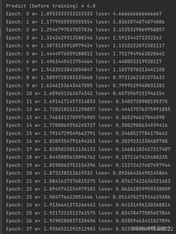
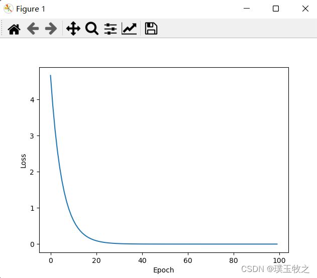
1.4 结果截图

2.Stochastic Gradient Descent (随机梯度下降)

由于损失函数可能是带有鞍点的，到达鞍点后就无法继续向前走了。我们拿到的数据总是有噪声的，在陷入鞍点时，随机噪声可能会把我们向前推动。

引入随机性后，在更新时，有可能跨过鞍点向最优值前进。

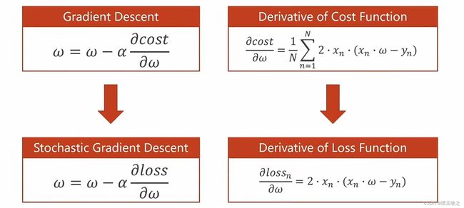
梯度下降是用所有样本的平均损失作为梯度下降的更新依据，随机梯度下降是一共提供N个数据，从里面随机选一个，公式就变成了拿单个样本的损失函数对权重求导。

2.1 代码实现

import matplotlib.pyplot as plt

x_data = [1.0, 2.0, 3.0]
y_data = [2.0, 4.0, 6.0]  #输入训练集数据

w = 1.0

def forward(x):           #定义前馈计算
    return x * w

def loss(x, y):
    y_pred = forward(x)  # 计算y_hat=x*w
    return (y_pred - y) ** 2  #计算y_hat-y的平方

def gradient(x, y):      #求梯度函数
    return 2 * x * (x * w - y)

epoch_list = []
loss_list = []

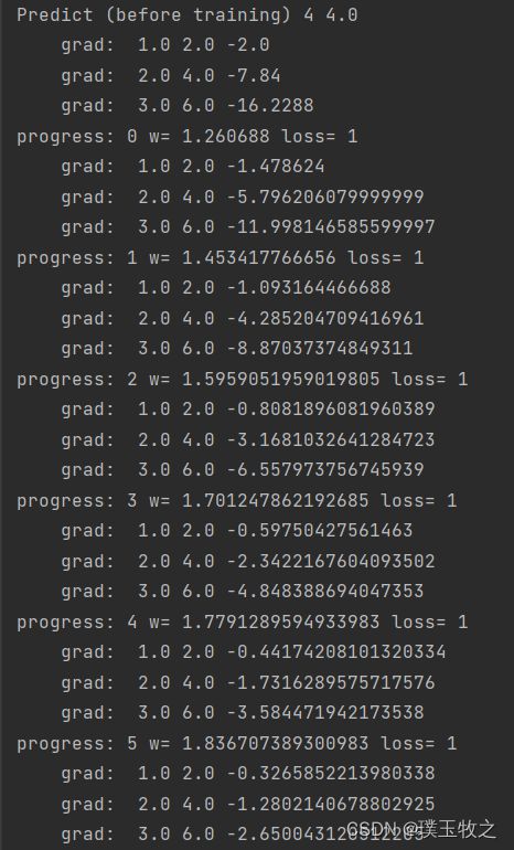
print('Predict (before training)', 4, forward(4))
for epoch in range(100):
    for x, y in zip(x_data, y_data):
        grad = gradient(x, y) #对每个样本求梯度
        w = w - 0.01 * grad   #拿一个样本然后就进行更新权重
        print("\tgrad: ", x, y, grad)
        l = loss(x, y)

    print("progress:", epoch, "w=", w, "loss=", 1)

    epoch_list.append(epoch)
    loss_list.append(l)

print('Predict (after training)', 4, forward(4))

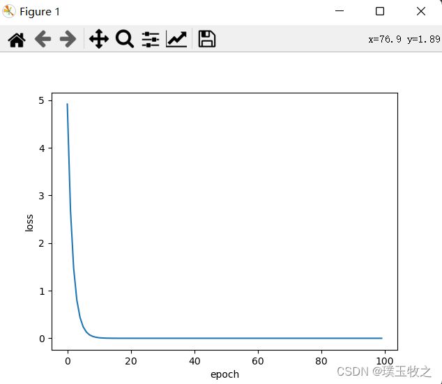
#Draw the grap
plt.plot(epoch_list, loss_list)
plt.ylabel('loss')
plt.xlabel('epoch')
plt.show()

2.2 结果截图

3.Batch (批量的随机梯度下降)

• 梯度下降的计算是并行的，随机梯度下降的两个样本之间是有依赖的，不能并行。所以，梯度下降法效率最高，随机梯度下降的性能较好，但时间复杂度高。
• 因此在深度学习中，会利用一种折中方式——Batch，批量的随机梯度下降（若干个样本一组，每次用一组样本求相应梯度，然后进行更新）
• 在深度学习中默认采用的随机梯度下降sdd算法用的就是batch方法。

本文参考：《PyTorch深度学习实践》