数字图像处理 形态学运算&逆滤波

1. 读取图像img1.tif，对其进行腐蚀操作；读取图像img2.tif，对其进行膨胀操作；读取图像img3.tif对其进行开运算和闭运算，结构元大小可自定。

   A=imread('C:\Users\hp\Desktop\img1.tif');
   figure,subplot(221),imshow(A),title('原始图片');
   se=strel('square',15);   % 生成方形结构元素
   A1=imerode(A,se);    %   腐蚀
   subplot(222),imshow(A1)
   title('腐蚀'); 
   
   B=imread('C:\Users\hp\Desktop\img2.tif');
   subplot(223),imshow(B),title('原始图片');
   se=strel('square',15);   % 生成方形结构元素
   B1=imdilate(B,se);    %   膨胀
   subplot(224),imshow(B1)
   title('膨胀');
   
   C=imread('C:\Users\hp\Desktop\img3.tif');
   figure,subplot(221),imshow(A)
   title('原始图片');
   se=strel('square',15);   % 生成方形结构元素
   C1=imopen(C,se);    %   膨胀
   subplot(222),imshow(C1),title('直接开运算');
   C2=imclose(C,se);
   subplot(223),imshow(C2),title('直接闭运算');

 

 

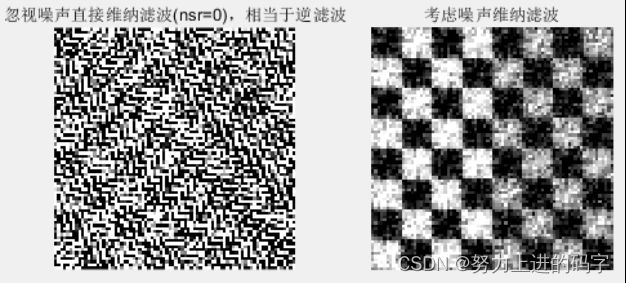
2.生成棋盘图像，通过运动模糊（len = 7, theta = -45°）和高斯噪声（theta = sqrt(0.001)）生成其退化图像。随后计算其逆滤波和维纳滤波结果。

clc;        
clear;       
close all;   
I=checkerboard(10);%生成棋盘图像
subplot(131),imshow(I);

H_motion = fspecial('motion', 7, -45);%运动长度为7，逆时针运动角度为-45°
motion_blur = imfilter(I, H_motion, 'conv', 'circular');%加入运动模糊

noise_mean=0;  %添加均值为0
noise_var=0.001; %方差为0.001的高斯噪声
motion_blur_noise=imnoise(motion_blur,'gaussian',noise_mean,noise_var);%添加均值为0，方差为0.001的高斯噪声
subplot(1,3,2);imshow(motion_blur,[]);title('运动模糊');
subplot(1,3,3);imshow(motion_blur_noise,[]);title('运动模糊添加噪声');
restore_ignore_noise = deconvwnr(motion_blur_noise, H_motion, 0); 

signal_var=var(I(:));
estimate_nsr=noise_var/signal_var;   %噪信比估值
restore_with_noise=deconvwnr(motion_blur_noise,H_motion,estimate_nsr);  %信号的功率谱使用图像的方差近似估计
figure('name','函数法维纳滤波');
subplot(1,2,1);imshow(im2uint8(restore_ignore_noise),[]);title('忽视噪声直接维纳滤波(nsr=0)，相当于逆滤波');
subplot(1,2,2);imshow(im2uint8(restore_with_noise),[]);title('考虑噪声维纳滤波');

 

 

 3.分别通过sobel算子, prewitt算子, roberts算子, log算子, canny算子，完成图像img4.tif和img5.tif的边缘检测。

clear;clc; 
%读取图像
I=imread('C:\Users\hp\Desktop\img4.tif');
h=fspecial('gaussian',5);%高斯滤波
I2=imfilter(I,h,'replicate');
GsobelBW=edge(I2,'sobel');%高斯滤波后使用sobel算子进行边缘检测
GprewittBW=edge(I2,'prewitt');
GrobertsBW=edge(I2,'roberts');
GlogBW=edge(I2,'log');
GcannyBW=edge(I2,'canny');
subplot(231),imshow(I,[]);title('Original Image');
subplot(232),imshow(GsobelBW);title('Gaussian & sobel Edge');
subplot(233),imshow(GprewittBW);title('Gaussian & perwitt Edge');
subplot(234),imshow(GrobertsBW);title('Gaussian & roberts Edge');
subplot(235),imshow(GlogBW);title('Gaussian & log Edge');
subplot(236),imshow(GcannyBW);title('Gaussian & Canny Edge');