GTSAM中imu预积分及其因子图优化过程

前言

使用IMU和llidar或者相机进行多传感器融合的slam方案中，主要分为紧耦合和松耦合方案。目前，主流的方案都是紧耦合的。而紧耦合方案中主要分为基于滤波（比如，ESKF）和基于优化的方案。
本文则介绍基于优化方案中IMU的预积分理论以及其在GTSAM中的实现。

IMU预积分理论：

简介

IMU的使用一般是对其测得的加速度，角速度进行积分，从而推算出机器人的位姿。但是，由于积分关系，IMU的积分所得的位姿飘移会随着积分时间的增大而增大。另一方面，当优化方法优化了历史时刻的位姿之后，之后时刻的IMU积分值需要重新进行积分，计算量大。因此，IMU预积分就被提出，以解决以上问题。IMU预积分简单来说就是描述了lidar帧（或者相机帧）之间（时间间隔比较短，比如lidar帧间间隔通常为100ms），IMU数据的观测量。其只跟上一帧时刻的IMU状态量相关，因此，在进行优化过程中，计算量较小。作为观测量，IMU预积分自然是作为一个约束用于slam位姿优化。

公式推导

IMU模型：

其中，$w^b$是IMU坐标系中角速度的真实值。$a^w$是世界坐标系中加速度真实值。$b^g$,$b^a$为IMU偏置，用随机游走建模。$n^g$,$n^a$为测量值的噪声。$a^b$,$w^b$为IMU测量值。
根据积分关系，可以得到位置，速度和姿态的迭代公式。

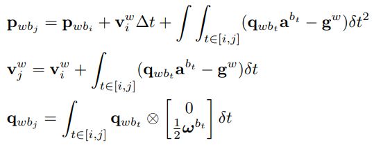
又因为

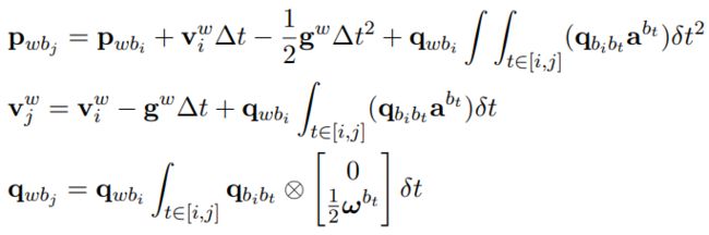
那么，PVQ积分公式中的积分项则变为相对于第i时刻的姿态，而不是相对于世界坐标系的姿态：

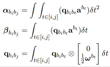
进而定义预积分量：

移项整理，构建残差：

此时，获得了优化过程中需要的残差，残差对相应的状态量求导可得雅可比矩阵。但是，缺少了优化过程需要的协方差矩阵。因此，需要推导出imu噪声协方差和预积分协方差的关系。
根据预积分的定义，使用中值积分方法对其进行离散化，可得：

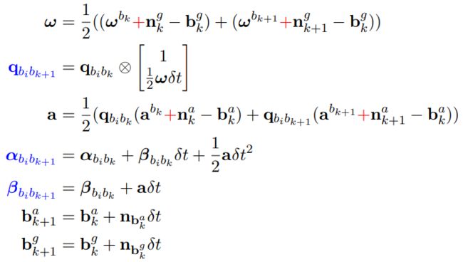
根据上式可以发现，预积分量和imu测量值之间是非线性关系，直接通过该方程求得协方差传播不现实，需要进行线性化。
根据EKF的线性化过程，对上述方程进行一阶泰勒展开，可得：

其中，F,G分别是方程$f(x_{k-1},u_{k-1})$在${\hat{x}}_{k-1}$,噪声项为0处的雅可比矩阵。
由于误差量的协方差矩阵和原随机变量的协方差矩阵相同。因此，预积分量的协方差矩阵可以通过F,G雅可比矩阵进行传播。

---

GTSAM中IMU预积分实现及其因子图构建

简介

gtsam是通过因子图这个模型实现优化的。因此，在使用gtsam解决一个优化问题时，就需要构建相应的因子图。
在因子图中，图的节点就是待优化的变量，因子就是相应的观测约束。而节点的值（初始值）需要一个类Value来保存。
gtsam优化过程简单描述就是优化方法（比如，GN，ISAM）调用因子图以及相应图节点的值，计算因子（观测约束）的残差，因子（观测约束）对相关图节点（相关量）的雅可比，完成迭代优化。
因此，gtsam中因子的类（比如，ImuFactor）会有相应的求取残差以及雅可比的函数（比如，linearize()函数，这个函数会被重载）。

IMU预积分类

gtsam中的一种IMU预积分实现类是PreintegratedImuMeasurements。其中，

void PreintegrationBase::integrateMeasurement(const Vector3& measuredAcc,
    const Vector3& measuredOmega, double dt) {
  Matrix9 A;
  Matrix93 B, C;
  update(measuredAcc, measuredOmega, dt, &A, &B, &C);
}

这个成员函数，接受IMU的加速度，角速度测量值以及imu测量值之间的时间间隔。然后，计算相应的预积分量和噪声传播的雅克比矩阵。

NavState PreintegrationBase::predict(const NavState& state_i,
    const imuBias::ConstantBias& bias_i, OptionalJacobian<9, 9> H1,
    OptionalJacobian<9, 6> H2) const {
  Matrix96 D_biasCorrected_bias;
  Vector9 biasCorrected = biasCorrectedDelta(bias_i,
                                             H2 ? &D_biasCorrected_bias : nullptr);

  Matrix9 D_delta_state, D_delta_biasCorrected;
  Vector9 xi = state_i.correctPIM(biasCorrected, deltaTij_, p().n_gravity,
                                  p().omegaCoriolis, p().use2ndOrderCoriolis, H1 ? &D_delta_state : nullptr,
                                  H2 ? &D_delta_biasCorrected : nullptr);

  Matrix9 D_predict_state, D_predict_delta;
  NavState state_j = state_i.retract(xi,
                                     H1 ? &D_predict_state : nullptr,
                                     H2 || H2 ? &D_predict_delta : nullptr);
  if (H1)
    *H1 = D_predict_state + D_predict_delta * D_delta_state;
  if (H2)
    *H2 = D_predict_delta * D_delta_biasCorrected * D_biasCorrected_bias;
  return state_j;
}

这个成员函数根据预积分量以及输入的PVQ,Bias进行当前时刻imu积分值计算。计算得到的结果可以作为相应节点的初始值。

gtsam因子图构建

NonlinearFactorGraph* graph = new NonlinearFactorGraph();
graph->addPrior(X(correction_count), prior_pose, pose_noise_model);
graph->addPrior(V(correction_count), prior_velocity, velocity_noise_model);
graph->addPrior(B(correction_count), prior_imu_bias, bias_noise_model);

先实例化因子图对象，而后加入先验节点。

std::shared_ptr<PreintegrationType> preintegrated =
    std::make_shared<PreintegratedImuMeasurements>(p, prior_imu_bias);

创建imu预积分对象。

// Adding the IMU preintegration.
preintegrated->integrateMeasurement(imu.head<3>(), imu.tail<3>(), dt);

根据imu观测值的输入，进行imu预积分计算。直到获得位姿观测值。

auto preint_imu =
  dynamic_cast<const PreintegratedImuMeasurements&>(*preintegrated);
ImuFactor imu_factor(X(correction_count - 1), V(correction_count - 1),
                   X(correction_count), V(correction_count),
                   B(correction_count - 1), preint_imu);
graph->add(imu_factor);
imuBias::ConstantBias zero_bias(Vector3(0, 0, 0), Vector3(0, 0, 0));
graph->add(BetweenFactor<imuBias::ConstantBias>(
  B(correction_count - 1), B(correction_count), zero_bias,
  bias_noise_model));

当获得位姿观测值（比如，GPS数据，lidar匹配的位姿等）时，就利用imu预积分对象构建imu因子。

auto correction_noise = noiseModel::Isotropic::Sigma(3, 1.0);
GPSFactor gps_factor(X(correction_count),
                     Point3(gps(0),   // N,
                            gps(1),   // E,
                            gps(2)),  // D,
                     correction_noise);
graph->add(gps_factor);

同时，利用位姿观测值构建相应的因子。
至此，构建的因子图，如下所示：

其中，X节点是位姿，V节点是速度，B节点是bias。
然后，创建优化方法类对象，使用构建的因子图和初始值进行迭代优化。

LevenbergMarquardtOptimizer optimizer(*graph, initial_values);
result = optimizer.optimize();

---

GTSAM因子图优化源码实现：

gtsam中NonlinearConjugateGradientOptimizer这个优化器的optimize()源码如下所示：

const Values& NonlinearConjugateGradientOptimizer::optimize() {
  System system(graph_);
  Values newValues;
  int iterations;
  boost::tie(newValues, iterations) =
      nonlinearConjugateGradient(system, state_->values, params_, false);
  state_.reset(new State(std::move(newValues), graph_.error(newValues), iterations));
  return state_->values;
}

其中，nonlinearConjugateGradient函数就是调用因子图中的因子类对象，计算残差和相应的雅可比矩阵。然后，使用该优化器的优化算法进行节点变量优化。具体说明雅可比矩阵的实现过程。

static VectorValues gradientInPlace(const NonlinearFactorGraph &nfg,
    const Values &values) {
  // Linearize graph
  GaussianFactorGraph::shared_ptr linear = nfg.linearize(values);
  return linear->gradientAtZero();
}

其中，主要是因子图对象调用linearize()函数。linearize()函数部分源码如下所示：

GaussianFactorGraph::shared_ptr NonlinearFactorGraph::linearize(const Values& linearizationPoint) const
{
  gttic(NonlinearFactorGraph_linearize);

  // create an empty linear FG
  GaussianFactorGraph::shared_ptr linearFG = boost::make_shared<GaussianFactorGraph>();

#ifdef GTSAM_USE_TBB

  linearFG->resize(size());
  TbbOpenMPMixedScope threadLimiter; // Limits OpenMP threads since we're mixing TBB and OpenMP

  // First linearize all sendable factors
  tbb::parallel_for(tbb::blocked_range<size_t>(0, size()),
    _LinearizeOneFactor(*this, linearizationPoint, *linearFG));

  // Linearize all non-sendable factors
  for(size_t i = 0; i < size(); i++) {
    auto& factor = (*this)[i];
    if(factor && !(factor->sendable())) {
      (*linearFG)[i] = factor->linearize(linearizationPoint);
    }
  }
  return linearFG;
}

其中，有使用tbb多线程，访问因子图中的因子，调用因子对象中的linearize()函数。而对于ImuFactor这个因子对象，由于其是NoiseModelFactor的子类。因此，调用了NoiseModelFactor的linearize()函数，其源码如下所示：

boost::shared_ptr<GaussianFactor> NoiseModelFactor::linearize(
    const Values& x) const {

  // Only linearize if the factor is active
  if (!active(x))
    return boost::shared_ptr<JacobianFactor>();

  // Call evaluate error to get Jacobians and RHS vector b
  std::vector<Matrix> A(size());
  Vector b = -unwhitenedError(x, A);
  check(noiseModel_, b.size());

  // Whiten the corresponding system now
  if (noiseModel_)
    noiseModel_->WhitenSystem(A, b);

  // Fill in terms, needed to create JacobianFactor below
  std::vector<std::pair<Key, Matrix> > terms(size());
  for (size_t j = 0; j < size(); ++j) {
    terms[j].first = keys()[j];
    terms[j].second.swap(A[j]);
  }

  // TODO pass unwhitened + noise model to Gaussian factor
  using noiseModel::Constrained;
  if (noiseModel_ && noiseModel_->isConstrained())
    return GaussianFactor::shared_ptr(
        new JacobianFactor(terms, b,
            boost::static_pointer_cast<Constrained>(noiseModel_)->unit()));
  else
    return GaussianFactor::shared_ptr(new JacobianFactor(terms, b));
}

而其中的unwhitenedError函数，则是计算残差和雅可比矩阵的函数，该函数最终调用imu预积分类PreintegratedImuMeasurements中的残差计算，雅可比矩阵求导函数computeErrorAndJacobians。
至此，摸索清楚了从优化器到残差，雅可比矩阵计算的整个计算流程。
才疏学浅，如有错误，欢迎批评指正！