Pytorch损失函数解析

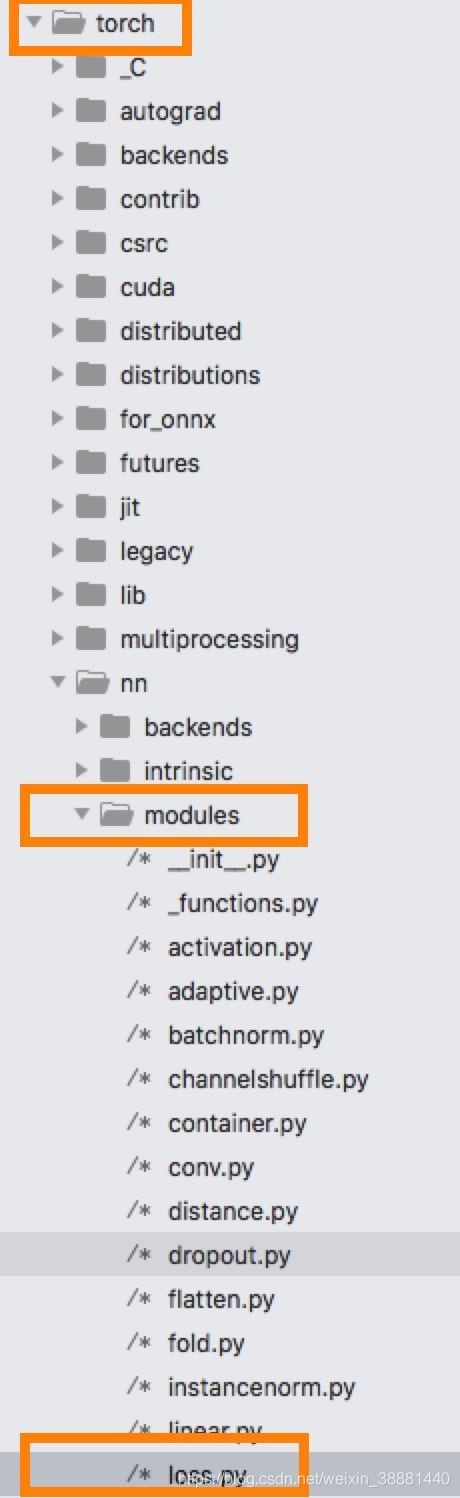
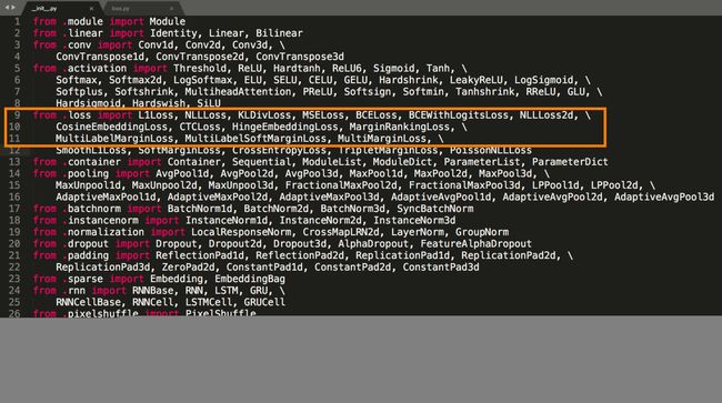
本文根据pytorch里面的源码解析各个损失函数，各个损失函数的python接口定义于包torch.nn.modules中的loss.py，在包modules的初始化__init__.py中关于损失函数的导入:

1.损失函数的base类

1.1 Loss的三个参数

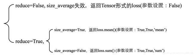
​ 从函数代码中可以看出，__init__函数有三个参数size_average, reduce, reduction，这三个参数的关系如下图所示；可以很明显看出，reduce参数控制返回的是Tensor还是scalar，size_average控制在一个batch里面的计算结果，根据需求可以自己设置，一般是(loss.mean())

​

2.1 weight

​ weight普遍用于分类任务，是一个长度和类别数目一样的Tensor，用于计算损失时针对不同类别进行加权，如下是数字识别不同数字损失的加权例子；

​

2.各个损失函数汇总

2.1 MAE(L1 Loss)

​ y是模型的预测输出，t是ground truth，两者都是长度为n的tensor，损失计算如下：

​
$$L(\mathbf{y},\mathbf{t})=\frac{1}{n}\sum _i^n|y_i-t_i|$$

2.2 MSE(L2 Loss)

​ y是模型的预测输出，t是ground truth，两者都是长度为n的tensor，损失计算如下：
$$L(\mathbf{y},\mathbf{t})=\frac{1}{n}\sum _i^n|y_i-t_i{|}^2$$

2.3 BCELoss & BCEWithLogitsLoss

​ BCELoss是常用于二分类的损失函数，y是模型的预测输出(sigmoid的概率值)，t是ground truth标签(非0即1)，损失计算如下：

​
$$L(\mathbf{y},\mathbf{t})=-\frac{1}{n}\sum _i^n(t_i\cdot \log y_i+(1-t_i)\cdot \log (1-y_i))$$
​

​ BCEWithLogitsLoss=Sigmoid+BCELoss，不需要在模型输出添加sigmoid层，因为这部分已经被包含在损失函数内部；

2.4 NLLLoss

​ 分类损失：LogSoftmax + NLLLoss = CrossEntropyLoss

​ y是模型的预测输出(LogSoftmax的值(-∞,0))，t是ground truth标签，损失计算如下：

​
$$L(\mathbf{y},\mathbf{t})=-\frac{1}{n}\sum _i^n{y}_i[t_i]$$
​ 举个例子，比如经过LogSoftmax的输出Tensor为[-1.233, -2.657,-0.534]，label为2，则损失为0.534。

2.5 CrossEntropyLoss

​ y是模型的预测输出，是长度为类别数量n的tensor，t是ground truth标签，损失计算如下：

​
$$L(\mathbf{y},\mathbf{t})=-\log (\frac{exp(y_{\mathbf{t}})}{{\sum }_{j}exp(y_j)})$$

2.6 MultiLabelMarginLoss

​ y是模型的预测输出，是长度为类别数量n的tensor，t是ground truth标签(one-hot编码)，损失计算如下：
$$L(\mathbf{y},\mathbf{t})=\sum _{ij}\frac{max(0,1-(t[y[j]]-y[i]))}{y.size(0)}$$

2.7 MultiLabelSoftMarginLoss

​ y是模型的预测输出，是长度为类别数量n的tensor，t是ground truth标签(one-hot编码)，损失计算如下：

​
$$L(\mathbf{y},\mathbf{t})=-\sum _i(t[i]\ast \log (1+exp(-y[i]){)}^{-1}+(1-t[i])\ast \log (\frac{exp(-y[i])}{(1+exp(-y[i])}))$$

2.8 MultiMarginLoss

​ y是模型的预测输出，是长度为类别数量n的tensor，t是ground truth标签(one-hot编码)，损失计算如下：

​
$$L(\mathbf{y},\mathbf{t})=\frac{{\sum }_{i}max(0,w[t]\ast (margin-y[t]+y[i]{)}^p)}{y.size(0)}$$

2.9 SoftMarginLoss

​ y是模型的预测输出，是长度为类别数量n的tensor，t是ground truth标签(二分类，-1或1)，损失计算如下：

​
$$L(\mathbf{y},\mathbf{t})=\sum _i\frac{\log (1+exp(-t[i]\ast y[i]))}{y.nelement()}$$
​

2.10 SmoothL1Loss

​ Huber Loss常用于回归问题，对离群点，噪声不敏感，y是模型的预测输出，t是ground truth，两者都是长度为n的tensor,损失函数如下，

​
$$L_{\delta }({\mathbf{y}}_{\mathbf{i}},{\mathbf{t}}_{\mathbf{i}})=\{\begin{array}{ll}\frac{1}{2}({\mathbf{y}}_{\mathbf{i}}-{\mathbf{t}}_{\mathbf{i}}{)}^2& |{\mathbf{y}}_{\mathbf{i}}-{\mathbf{t}}_{\mathbf{i}}|<\delta \\ \delta |{\mathbf{y}}_{\mathbf{i}}-{\mathbf{t}}_{\mathbf{i}}|-\frac{1}{2}{\delta }^2& otherwise\end{array}$$
​
$$L_{\delta }(\mathbf{y},\mathbf{t})=\frac{1}{n}\sum _{i=1}^n{L}_{\delta }({\mathbf{y}}_{\mathbf{i}},{\mathbf{t}}_{\mathbf{i}})$$
SmoothL1Loss是Huber Loss函数特殊化，\delta=1时，
$$L_{smoothl1}({\mathbf{y}}_{\mathbf{i}},{\mathbf{t}}_{\mathbf{i}})=\{\begin{array}{ll}\frac{1}{2}({\mathbf{y}}_{\mathbf{i}}-{\mathbf{t}}_{\mathbf{i}}{)}^2& |{\mathbf{y}}_{\mathbf{i}}-{\mathbf{t}}_{\mathbf{i}}|<1\\ |{\mathbf{y}}_{\mathbf{i}}-{\mathbf{t}}_{\mathbf{i}}|-\frac{1}{2}& otherwise\end{array}$$

$$L_{smoothl1}(\mathbf{y},\mathbf{t})=\frac{1}{n}\sum _{i=1}^n{L}_{smoothl1}({\mathbf{y}}_{\mathbf{i}},{\mathbf{t}}_{\mathbf{i}})$$
​

2.11 KLDivLoss

​ K-L源于信息论，信息量的度量单位是熵，一般用H来表示，分布的熵的公式如下：
$$H=-\sum _{i=1}^{N}p(x_i)\log p(x_i)$$
​ 只需要改进一下H的公式，就能得到k-L散度的计算公式，设p为观察得到的概率分布，q是另一分布来近似p，则p,q之间的K-L散度为：

​
$$D(p_i||q_i)=\sum _{i=1}^{n}p(x_i)\cdot (\log p(x_i)-\log q(x_i))=\sum _{i=1}^{n}p(x_i)\log (\frac{p(x_i)}{q(x_i)})$$
​ 需要注意的是，K-L散度并不是不同分布之间距离的度量，因为从计算公式来看，是不满足对称性！

2.12 MarginRankingLoss

​ 计算两个张量的相似度，输入是三个参数，x1，x2以及y是长度相同的Tensor，y取值为-1或者1，
$$L(x_1,x_2,y)=max(0,-y\ast (x_1-x_2)+margin)=\{\begin{array}{ll}max(0,-(x_1-x_2)+margin)& y=1\\ max(0,(x_1-x_2)+margin)& y=-1\end{array}$$

2.13 CosineEmbeddingLoss

​ 余弦损失函数，计算两个向量的相似性，两个向量的余弦值越高，则相似性越高，输入是三个参数，x1，x2以及y是长度相同的Tensor，y取值为-1或者1，

​
$$L(x_1,x_2,y)=\{\begin{array}{ll}1-cos(x_1,x_2)& y=1\\ max(0,cos(x_1-x_2)-margin)& y=-1\end{array}$$
​ 1.当y=1时，直接用-cos(x1,x2)的平移函数作为损失函数；

​ 2.当y=-1时，在cos(x1,x2)=margin处做了分割，用于衡量两个向量的不相似性；

2.14 HingeEmbeddingLoss

​ 输入是两个参数，x与y是长度相同的Tensor，y取值为-1或者1，

​
$$loss(x,y)=\frac{1}{n}\sum _{i=1}^n\{\begin{array}{ll}{x}_i& y_i=1\\ max(0,margin-x_i)& y_i=-1\end{array}$$
​ margin默认为1，

​ 1.当y=-1的时候，loss=max(0,1-x)，如果x>1(margin)，则loss=0；如果x<1，则loss=1-x;

​ 2.当y=1，loss=x。

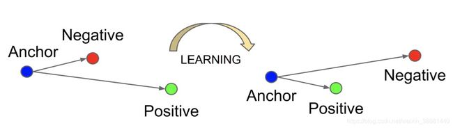
2.15 TripletMarginLoss

​ Triplet Loss是用来训练差异性较小的样本，如人脸等，数据选择包括三项Anchor示例，Positive示例，Negative示例，通过优化Anchor示例与正示例的距离小于Anchor示例与负示例的距离，来实现样本的相似性的计算，如下图所示：

​

​ 损失函数如下：

​
$$L(a,p,n)=\frac{1}{n}\sum _{i=1}^{n}max\{d(a_i,p_i)-d(a_i,n_i)+margin,0\}$$
​
$$d(x_i,y_i)=||x_i-y_i|{|}_p$$

3.参考说明：

​ 本文是作者在实践过程中总结出来的激活函数说明，后续有补充会及时更新，如有不正确之处，欢迎各位大佬批评指正！！！

​ 1.https://www.jianshu.com/p/43318a3dc715;

​ 2.https://juejin.cn/post/6844903949124763656;

​ 3.https://www.jianshu.com/p/46c6f68264a1;

​ 4.https://my.oschina.net/u/4584682/blog/4481019