SNN(脉冲神经网络)——Brian2_STDP_MNIST学习记录

这篇是学习Brian2模拟器一个手写数字识别的代码学习记录

我非常想结识相关领域的朋友，大家感兴趣可以看到最后一段。
本文参考：建议先读一下这篇论文和过一遍Brian2的使用手册。

Peter, U, Diehl, et al. Unsupervised learning of digit recognition using spike-timing-dependent plasticity[J]. Frontiers in Computational Neuroscience, 2015, 9:99.
https://brian2.readthedocs.io/en/stable/index.html

本文源代码工程地址：
https://github.com/zxzhijia/Brian2STDPMNIST

（一）前置基本函数

第一个功能函数get_labeled_data:

def get_labeled_data(picklename, bTrain = True):
    """Read input-vector (image) and target class (label, 0-9) and return
       it as list of tuples.
    """
    if os.path.isfile('%s.pickle' % picklename):
        data = pickle.load(open('%s.pickle' % picklename))
    else:
        # Open the images with gzip in read binary mode
        if bTrain:
            images = open(MNIST_data_path + 'train-images.idx3-ubyte','rb')
            labels = open(MNIST_data_path + 'train-labels.idx1-ubyte','rb')
        else:
            images = open(MNIST_data_path + 't10k-images.idx3-ubyte','rb')
            labels = open(MNIST_data_path + 't10k-labels.idx1-ubyte','rb')
        # Get metadata for images
        images.read(4)  # skip the magic_number
        number_of_images = unpack('>I', images.read(4))[0]
        rows = unpack('>I', images.read(4))[0]
        cols = unpack('>I', images.read(4))[0]
        # Get metadata for labels
        labels.read(4)  # skip the magic_number
        N = unpack('>I', labels.read(4))[0]

        if number_of_images != N:
            raise Exception('number of labels did not match the number of images')
        # Get the data
        x = np.zeros((N, rows, cols), dtype=np.uint8)  # Initialize numpy array
        y = np.zeros((N, 1), dtype=np.uint8)  # Initialize numpy array
        for i in xrange(N):
            if i % 1000 == 0:
                print("i: %i" % i)
            x[i] = [[unpack('>B', images.read(1))[0] for unused_col in xrange(cols)]  for unused_row in xrange(rows) ]
            y[i] = unpack('>B', labels.read(1))[0]

        data = {'x': x, 'y': y, 'rows': rows, 'cols': cols}
        pickle.dump(data, open("%s.pickle" % picklename, "wb"))
    return data

该函数主要功能为，读取MNIST数据集，并将其各个参数依次读出，如图片个数，每一张图片的大小，MNIST数据集为28✖28，并将像素数据存入np的矩阵中。在第一次运行该函数的时候，会自动生成pickle文件，那样下一次就不用继续的MNIST数据集的了，可直接读配置好的pickle文件。

第二个功能函数：get_matrix_from_file

这个函数看名字就知道是从disk的file里读取矩阵，其实也就是权重矩阵。
源码如下：（为了函数功能清楚，调试时加了点code）

MNIST_data_path = ''
ending = ''
n_input = 784
n_e = 10
n_i = 10
def get_matrix_from_file(fileName):#
    offset = len(ending) + 4#4
    if fileName[-4-offset] == 'X':
        n_src = n_input
    else:
        if fileName[-3-offset]=='e':
            n_src = n_e
        else:
            n_src = n_i
    if fileName[-1-offset]=='e':
        n_tgt = n_e
    else:
        n_tgt = n_i
    print offset,n_src,n_tgt
    readout = np.load(fileName)
    print readout.shape, fileName
    value_arr = np.zeros((n_src, n_tgt))
    if not readout.shape == (0,):
        print "YES"
        value_arr[np.int32(readout[:,0]), np.int32(readout[:,1])] = readout[:,2]
    return value_arr
if __name__ == "__main__":
    x = get_matrix_from_file("random/AiAe.npy")
    print x

代码中出现了offset这个偏移量，其实是取决于从disk中读取文件的文件所决定的，主要是判断当前权重是已经训练完成的权重，还是随机初始化。因为这个工程是根据2015年的一篇论文写出来的，如下：

Peter, U, Diehl, et al. Unsupervised learning of digit recognition using spike-timing-dependent plasticity[J]. Frontiers in Computational Neuroscience, 2015, 9:99.

论文中提出的SNN网络输入层与学习层全连接且均为兴奋性神经元，并增加了侧抑制功能，即学习层与侧抑制层一 一连接，侧抑制神经元连接除源神经元以外的神经元。看下面我调试的图片就很清楚了。（我缩小了网络规模，学习层10个神经元，侧抑制层10个神经元）。

读取“random/AeAi.npy”即学习层到侧抑制层的连接。

读取“random/AiAe.npy”即侧抑制层到学习层的连接。

仔细看结果应该就很容易理解了

第三个功能函数：save_connections

源码为：

def save_connections(ending = ''):
    print 'save connections'
    for connName in save_conns:#XeAe
        conn = connections[connName]
        connListSparse = zip(conn.i, conn.j, conn.w)
        np.save(data_path + 'weights/' + connName + ending, connListSparse)

该函数功能较简单，主要作用为：网络训练完成后，将训练好的权值放到disk的文件里。

第四个功能函数：save_theta

源码为：

def save_theta(ending = ''):
    print 'save theta'
    for pop_name in population_names:
        np.save(data_path + 'weights/theta_' + pop_name + ending, neuron_groups[pop_name + 'e'].theta)

该函数与上一个函数功能相似，均为训练完成后使用，这个theta值是调整神经元膜电位的，论文中有提到它的训练方法。

第五个功能函数：normalize_weights

def normalize_weights():
    for connName in connections:
        if connName[1] == 'e' and connName[3] == 'e':# XeAe : Input and Exact
            len_source = len(connections[connName].source)#784
            len_target = len(connections[connName].target)#400
            connection = np.zeros((len_source, len_target))#784 * 400
            connection[connections[connName].i, connections[connName].j] = connections[connName].w#set the weights of connection to array
            temp_conn = np.copy(connection)# copy a array
            colSums = np.sum(temp_conn, axis = 0)# sum of all weights
            colFactors = weight['ee_input']/colSums # normalize parameter
            for j in range(n_e):
                temp_conn[:,j] *= colFactors[j]  # normalize
            connections[connName].w = temp_conn[connections[connName].i, connections[connName].j] #update the weights of connections

整体上理解，就是将权值进行正则化，会定义一个正则化的值，通过求和，得到正则化参数，将每一个weight乘上这个参数，依次来正则化权值，具体这样做的原因，论文有提到一篇引文，准备去看看。

第六个功能函数：get_2d_input_weights

源码：（我稍稍注释了一下）

def get_2d_input_weights():
    name = 'XeAe'
    weight_matrix = np.zeros((n_input, n_e))# 784 * 400
    n_e_sqrt = int(np.sqrt(n_e)) # 20
    n_in_sqrt = int(np.sqrt(n_input)) # 28
    num_values_col = n_e_sqrt*n_in_sqrt # 28 * 20
    num_values_row = num_values_col # 28 * 20
    rearranged_weights = np.zeros((num_values_col, num_values_row))# 560 * 560
    connMatrix = np.zeros((n_input, n_e)) # 784 * 400
    connMatrix[connections[name].i, connections[name].j] = connections[name].w # set the weights to the connMatrix
    weight_matrix = np.copy(connMatrix)# copy one

    for i in range(n_e_sqrt):# 20
        for j in range(n_e_sqrt): # 20 20*20
                rearranged_weights[i*n_in_sqrt : (i+1)*n_in_sqrt, j*n_in_sqrt : (j+1)*n_in_sqrt] = \
                    weight_matrix[:, i + j*n_e_sqrt].reshape((n_in_sqrt, n_in_sqrt)) # get a neuron 784 weights for 400 times
    return rearranged_weights

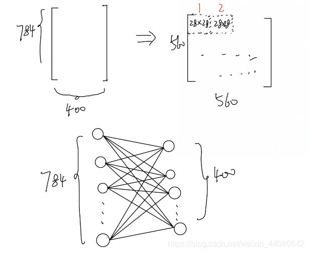
这个函数的主要功能个人认为就是一个矩阵转换，本来是一个输入对应400个权重，这个函数将其转换成400个28×28组成560*560的矩阵。这样就可以得到每一个学习层神经元的对应784个突触的权重了。如下图：具体的论文里的Section Result也有所提及。

第七个功能函数：plot_2d_input_weights

源码：

def plot_2d_input_weights():
    name = 'XeAe'
    weights = get_2d_input_weights()
    fig = b2.figure(fig_num, figsize = (18, 18))
    im2 = b2.imshow(weights, interpolation = "nearest", vmin = 0, vmax = wmax_ee, cmap = cmap.get_cmap('hot_r'))
    b2.colorbar(im2)
    b2.title('weights of connection' + name)
    fig.canvas.draw()
    return im2, fig

画出刚才转换而成的矩阵的图。

第八个功能函数：update_2d_input_weights

源码：

def update_2d_input_weights(im, fig):
    weights = get_2d_input_weights()
    im.set_array(weights)
    fig.canvas.draw()
    return im

第九个功能函数：get_current_performance

源码：

def get_current_performance(performance, current_example_num):
    current_evaluation = int(current_example_num/update_interval)
    start_num = current_example_num - update_interval
    end_num = current_example_num
    difference = outputNumbers[start_num:end_num, 0] - input_numbers[start_num:end_num]
    correct = len(np.where(difference == 0)[0])# if the result is 0,denote that recognize the right number
    performance[current_evaluation] = correct / float(update_interval) * 100 #get the accuracy
    return performance

这个函数是测试准确度的，有利于我们在测试训练网络的过程观察网络训练效果，主要方法我在代码中有标注出来。

第十、十一个函数一起看：plot_performance，update_performance_plot

其实这两个函数就是，画图、更新图。
源码如下：

def plot_performance(fig_num):
    num_evaluations = int(num_examples/update_interval)
    time_steps = range(0, num_evaluations)
    performance = np.zeros(num_evaluations)
    fig = b2.figure(fig_num, figsize = (5, 5))
    fig_num += 1
    ax = fig.add_subplot(111)
    im2, = ax.plot(time_steps, performance) #my_cmap
    b2.ylim(ymax = 100)
    b2.title('Classification performance')
    fig.canvas.draw()
    return im2, performance, fig_num, fig

def update_performance_plot(im, performance, current_example_num, fig):
    performance = get_current_performance(performance, current_example_num)
    im.set_ydata(performance)
    fig.canvas.draw()
    return im, performance

第十二个功能函数：get_recognized_number_ranking

源码：

def get_recognized_number_ranking(assignments, spike_rates):
    summed_rates = [0] * 10
    num_assignments = [0] * 10
    for i in range(10):
        num_assignments[i] = len(np.where(assignments == i)[0])# find the class is below to i (the number of neuron)
        if num_assignments[i] > 0:
            summed_rates[i] = np.sum(spike_rates[assignments == i]) / num_assignments[i]
    return np.argsort(summed_rates)[::-1] # from max to min because of [::-1]

首先需要知道，一共有400个输出神经元（也是学习神经元），所以论文中有提到，每一个神经元都会对应到一个类里面去。毕竟手写数字识别也是分类问题，共有10类。至于哪些神经元需要放到哪一类里面去呢，这个继续探讨。当前函数就是为了统计各个类的放电概率，并将其从大到小的排序，这样放电概率最大那个类，我们就认为是识别出的数字。

第十三个功能函数：get_new_assignments

源码为：

def get_new_assignments(result_monitor, input_numbers):
    assignments = np.zeros(n_e) # 400
    input_nums = np.asarray(input_numbers) #
    maximum_rate = [0] * n_e # 400
    for j in range(10):#10 numbers
        num_assignments = len(np.where(input_nums == j)[0])
        if num_assignments > 0:
            rate = np.sum(result_monitor[input_nums == j], axis = 0) / num_assignments
        for i in range(n_e):
            if rate[i] > maximum_rate[i]:
                maximum_rate[i] = rate[i]
                assignments[i] = j
    return assignments

上面有提到怎么吧神经元归类呢？上述函数就做到了这个事情。当调用这个函数的时候，需要有input_numbers以及result_monitor。分别代表输入到网络中的真实数字，以及经过网络运算后监视器的结果。根据当前数字的放电概率，采用循环依次刷新神经元所属类别。如下图：

（二）SNN 搭建

1、加载训练及测试数据集

#------------------------------------------------------------------------------
# load MNIST
#------------------------------------------------------------------------------
start = time.time()
training = get_labeled_data(MNIST_data_path + 'training') # load train data (train['x'] is the image data,and train['y'] is labels
end = time.time()
print('time needed to load training set:', end - start)

start = time.time()
testing = get_labeled_data(MNIST_data_path + 'testing', bTrain = False)# load train data (test['x'] is the image data,and test['y'] is labels
end = time.time()
print ('time needed to load test set:', end - start)

这里用到的是第一个函数，上面提到过。

2、基本参数配置（1）

test_mode = True

np.random.seed(0)
data_path = './'
if test_mode: # test mode
    weight_path = data_path + 'weights/'
    num_examples = 10000 * 1
    use_testing_set = True
    do_plot_performance = False
    record_spikes = True
    ee_STDP_on = False
    update_interval = num_examples
else:   # train mode
    weight_path = data_path + 'random/'
    num_examples = 60000 * 3
    use_testing_set = False
    do_plot_performance = True
    if num_examples <= 60000:
        record_spikes = True
    else:
        record_spikes = True
    ee_STDP_on = True


ending = ''
n_input = 784
n_e = 400
n_i = n_e

single_example_time =   0.35 * b2.second # one image train time 350ms
resting_time = 0.15 * b2.second # the reset time 150ms
runtime = num_examples * (single_example_time + resting_time)# all simmulation time

if num_examples <= 10000:
    update_interval = num_examples
    weight_update_interval = 20 # numbers of image
else:
    update_interval = 10000
    weight_update_interval = 100

if num_examples <= 60000:
    save_connections_interval = 10000
else:
    save_connections_interval = 10000
    update_interval = 10000

v_rest_e = -65. * b2.mV
v_rest_i = -60. * b2.mV

v_reset_e = -65. * b2.mV
v_reset_i = -45. * b2.mV

v_thresh_e = -52. * b2.mV
v_thresh_i = -40. * b2.mV

refrac_e = 5. * b2.ms
refrac_i = 2. * b2.ms

test_mode这个参数是选择网络是测试还是训练，True为测试，False为训练。还包含了如运行更新间隔，以及保存网络连接的间隔等。同时还有神经元模型的一些基本参数。

3、基本参数配置（2）

weight = {}
delay = {}
input_population_names = ['X']
population_names = ['A']
input_connection_names = ['XA']
save_conns = ['XeAe']
input_conn_names = ['ee_input']
recurrent_conn_names = ['ei', 'ie']
weight['ee_input'] = 78.
delay['ee_input'] = (0*b2.ms,10*b2.ms)
delay['ei_input'] = (0*b2.ms,5*b2.ms)
input_intensity = 2.
start_input_intensity = input_intensity

tc_pre_ee = 20*b2.ms
tc_post_1_ee = 20*b2.ms
tc_post_2_ee = 40*b2.ms

nu_ee_pre =  0.0001      # learning rate
nu_ee_post = 0.01       # learning rate

wmax_ee = 1.0
exp_ee_pre = 0.2
exp_ee_post = exp_ee_pre
STDP_offset = 0.4

这里我认为要理解代码描述网络的结构是什么样子的，我略微的画了一下，每个层，以及层与层之间的连接都是命好名字的，如图：

4、基本参数配置（3）

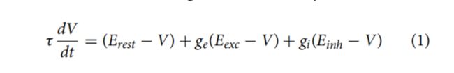
下面这一段代码个人认为比较重要，重要是理解论文中所提出的基于电导的LIF神经元模型，公式如下：具体的各个参数介绍，可以参考section 2.1。

代码如下：
关于神经元模型定义字符串那里，我稍稍写了一点备注。

if test_mode:
    scr_e = 'v = v_reset_e; timer = 0*ms'
else:
    tc_theta = 1e7 * b2.ms
    theta_plus_e = 0.05 * b2.mV
    scr_e = 'v = v_reset_e; theta += theta_plus_e; timer = 0*ms'
offset = 20.0*b2.mV
v_thresh_e_str = '(v>(theta - offset + v_thresh_e)) and (timer>refrac_e)'
v_thresh_i_str = 'v>v_thresh_i'
v_reset_i_str = 'v=v_reset_i'

# according to the equation in the paper , Eexc = 0mV , Einh = -100mV
# tau_e = 100ms
neuron_eqs_e = '''
        dv/dt = ((v_rest_e - v) + (I_synE+I_synI) / nS) / (100*ms)  : volt (unless refractory)
        I_synE = ge * nS *         -v                           : amp
        I_synI = gi * nS * (-100.*mV-v)                          : amp
        dge/dt = -ge/(1.0*ms)                                   : 1
        dgi/dt = -gi/(2.0*ms)                                  : 1
        '''
if test_mode:
    neuron_eqs_e += '\n  theta      :volt'
else:
    neuron_eqs_e += '\n  dtheta/dt = -theta / (tc_theta)  : volt'
neuron_eqs_e += '\n  dtimer/dt = 0.1  : second'

neuron_eqs_i = '''
        dv/dt = ((v_rest_i - v) + (I_synE+I_synI) / nS) / (10*ms)  : volt (unless refractory)
        I_synE = ge * nS *         -v                           : amp
        I_synI = gi * nS * (-85.*mV-v)                          : amp
        dge/dt = -ge/(1.0*ms)                                   : 1
        dgi/dt = -gi/(2.0*ms)                                  : 1
        '''
eqs_stdp_ee = '''
                post2before                            : 1
                dpre/dt   =   -pre/(tc_pre_ee)         : 1 (event-driven)
                dpost1/dt  = -post1/(tc_post_1_ee)     : 1 (event-driven)
                dpost2/dt  = -post2/(tc_post_2_ee)     : 1 (event-driven)
            '''
eqs_stdp_pre_ee = 'pre = 1.; w = clip(w + nu_ee_pre * post1, 0, wmax_ee)'
eqs_stdp_post_ee = 'post2before = post2; w = clip(w + nu_ee_post * pre * post2before, 0, wmax_ee); post1 = 1.; post2 = 1.'

5、基本参数配置（4）

以下代码的配置是学习层以及抑制层的生成，源码如下：

b2.ion()
fig_num = 1
neuron_groups = {}
input_groups = {}
connections = {}
rate_monitors = {}
spike_monitors = {}
spike_counters = {}
# just for updating the neuron's class ( from 0 - 9 )
result_monitor = np.zeros((update_interval,n_e))# 10000 * 400
# 400 exact neurons
neuron_groups['e'] = b2.NeuronGroup(n_e*len(population_names), neuron_eqs_e, threshold= v_thresh_e_str, refractory= refrac_e, reset= scr_e, method='euler')
# 400 inhib neurons
neuron_groups['i'] = b2.NeuronGroup(n_i*len(population_names), neuron_eqs_i, threshold= v_thresh_i_str, refractory= refrac_i, reset= v_reset_i_str, method='euler')

定义monitor和group我认为很重要，关于神经元群的定义可以去查阅brian2的官方手册，个人认为最好看英文版的，或者看手册中的代码，总体不是非常难。

（三）下面是这个工程几个比较重要的循环体：

第一个for：

for看起来好像是循环，其实只循环一次，当然只是针对这篇论文，感觉是可以配置成很多层网络的，有几层就会循环几次。
学习神经元层与侧抑制层的相互连接，在GitHub中，在issue中看到有人提出，这两个层之间是全连接，事实确实是如此。但这两层的连接依然符合论文中所提出的连接方法。（请看功能函数中提到的，没有连接的是以权重为0实现的）

#------------------------------------------------------------------------------
# create network population and recurrent connections
#------------------------------------------------------------------------------
for subgroup_n, name in enumerate(population_names):# ['A']
    print('create neuron group', name)

    neuron_groups[name+'e'] = neuron_groups['e'][subgroup_n*n_e:(subgroup_n+1)*n_e] # 400 neurons for 'Ae'
    neuron_groups[name+'i'] = neuron_groups['i'][subgroup_n*n_i:(subgroup_n+1)*n_e] # 400 neuron for 'Ai'

    neuron_groups[name+'e'].v = v_rest_e - 40. * b2.mV# set the initial potential
    neuron_groups[name+'i'].v = v_rest_i - 40. * b2.mV
    if test_mode or weight_path[-8:] == 'weights/':
        neuron_groups['e'].theta = np.load(weight_path + 'theta_' + name + ending + '.npy') * b2.volt # test mode , just load the theta file after training
    else:
        neuron_groups['e'].theta = np.ones((n_e)) * 20.0*b2.mV # train mode , just load random thera

    print('create recurrent connections')
    for conn_type in recurrent_conn_names:# ['ei','ie']
        connName = name+conn_type[0]+name+conn_type[1] # AeAi,AiAe
        weightMatrix = get_matrix_from_file(weight_path + '../random/' + connName + ending + '.npy')
        model = 'w : 1'
        pre = 'g%s_post += w' % conn_type[0] # ge_post , just flowing the paper
        post = ''
        if ee_STDP_on:
            if 'ee' in recurrent_conn_names:
                model += eqs_stdp_ee
                pre += '; ' + eqs_stdp_pre_ee
                post = eqs_stdp_post_ee
        connections[connName] = b2.Synapses(neuron_groups[connName[0:2]], neuron_groups[connName[2:4]],# Ae ---> Ai and Ai ----> Ae
                                                    model=model, on_pre=pre, on_post=post)
        connections[connName].connect(True) # all-to-all connection
        connections[connName].w = weightMatrix[connections[connName].i, connections[connName].j]

    print('create monitors for', name)
    rate_monitors[name+'e'] = b2.PopulationRateMonitor(neuron_groups[name+'e'])
    rate_monitors[name+'i'] = b2.PopulationRateMonitor(neuron_groups[name+'i'])
    spike_counters[name+'e'] = b2.SpikeMonitor(neuron_groups[name+'e'])

    if record_spikes:
        spike_monitors[name+'e'] = b2.SpikeMonitor(neuron_groups[name+'e'])
        spike_monitors[name+'i'] = b2.SpikeMonitor(neuron_groups[name+'i'])

两个层的连接思想我认为，首兴奋性神经元和抑制性神经元都在neuron_groups这个组里，那只需要配置突触的状态方程，关于突触的状态方程论文中虽然有提到几个模型，但是我没有在2015年这篇论文里找到代码中所提到的模型，可能与那一篇引文有关。
确定了突触模型（状态方程），我们就可以通过突触将这两层神经元相互连接了，最后配置权重即可，首先还是要掌握Brain2这个模拟器里Synapse的使用，很快的，啪的一下，就看的懂。

第二个for:

这个for，是生成泊松分布的输入脉冲，其实也就是输入数据的编码。这个原理有时间会单独说。

for i,name in enumerate(input_population_names):
    input_groups[name+'e'] = b2.PoissonGroup(n_input, 0*Hz) # poisson distribute , Hz
    rate_monitors[name+'e'] = b2.PopulationRateMonitor(input_groups[name+'e']) # record

第三个for：

这个for的功能和第一个for原理基本相同，也是将两层神经元连接，就不赘述了，不过要注意的是网络命名。

for name in input_connection_names:# ['XA'] , connect the input group and exact group
    print ('create connections between', name[0], 'and', name[1])
    for connType in input_conn_names:# ['ee_input']
        connName = name[0] + connType[0] + name[1] + connType[1] # XeAe
        weightMatrix = get_matrix_from_file(weight_path + connName + ending + '.npy')
        model = 'w : 1'
        pre = 'g%s_post += w' % connType[0]
        post = ''
        if ee_STDP_on:
            print ('create STDP for connection', name[0]+'e'+name[1]+'e')
            model += eqs_stdp_ee
            pre += '; ' + eqs_stdp_pre_ee
            post = eqs_stdp_post_ee

        connections[connName] = b2.Synapses(input_groups[connName[0:2]], neuron_groups[connName[2:4]],
                                                    model=model, on_pre=pre, on_post=post)
        minDelay = delay[connType][0]
        maxDelay = delay[connType][1]
        deltaDelay = maxDelay - minDelay
        # TODO: test this
        connections[connName].connect(True) # all-to-all connection
        connections[connName].delay = 'minDelay + rand() * deltaDelay'
        connections[connName].w = weightMatrix[connections[connName].i, connections[connName].j]

（四）网络搭建好，仿真开始

1、组建网络：

net = Network()
for obj_list in [neuron_groups, input_groups, connections, rate_monitors,
        spike_monitors, spike_counters]:
    for key in obj_list:
        net.add(obj_list[key])

这里是是Brain2里Network的用法，将上述定义的神经元、突触以及监听器等加入网络。

2、网络一些输入、输入变量定义：

previous_spike_count = np.zeros(n_e) # 400
assignments = np.zeros(n_e)
input_numbers = [0] * num_examples
outputNumbers = np.zeros((num_examples, 10))
if not test_mode:
    input_weight_monitor, fig_weights = plot_2d_input_weights()
    fig_num += 1
if do_plot_performance:
    performance_monitor, performance, fig_num, fig_performance = plot_performance(fig_num)
for i,name in enumerate(input_population_names):
    input_groups[name+'e'].rates = 0 * Hz
net.run(0*second)

包括记录上一次网络输出脉冲计数初始化，神经元分类，输入数据（0 - 9），输出数据（0 - 9）。

SNN网络训练或测试大循环（while）：

j = 0
while j < (int(num_examples)):# 60000 / 10000
    if test_mode:
        if use_testing_set:
            spike_rates = testing['x'][j%10000,:,:].reshape((n_input)) / 8. *  input_intensity
        else:
            spike_rates = training['x'][j%60000,:,:].reshape((n_input)) / 8. *  input_intensity
    else:
        normalize_weights()
        spike_rates = training['x'][j%60000,:,:].reshape((n_input)) / 8. *  input_intensity
    input_groups['Xe'].rates = spike_rates * Hz
#     print 'run number:', j+1, 'of', int(num_examples)
    net.run(single_example_time, report='text')

    if j % update_interval == 0 and j > 0:
        assignments = get_new_assignments(result_monitor[:], input_numbers[j-update_interval : j])
    if j % weight_update_interval == 0 and not test_mode:
        update_2d_input_weights(input_weight_monitor, fig_weights)
    if j % save_connections_interval == 0 and j > 0 and not test_mode:
        save_connections(str(j))
        save_theta(str(j))

    current_spike_count = np.asarray(spike_counters['Ae'].count[:]) - previous_spike_count
    previous_spike_count = np.copy(spike_counters['Ae'].count[:])
    if np.sum(current_spike_count) < 5:
        input_intensity += 1
        for i,name in enumerate(input_population_names):
            input_groups[name+'e'].rates = 0 * Hz
        net.run(resting_time)
    else:
        result_monitor[j%update_interval,:] = current_spike_count
        if test_mode and use_testing_set:
            input_numbers[j] = testing['y'][j%10000][0]
        else:
            input_numbers[j] = training['y'][j%60000][0]
        outputNumbers[j,:] = get_recognized_number_ranking(assignments, result_monitor[j%update_interval,:])
        if j % 100 == 0 and j > 0:
            print ('runs done:', j, 'of', int(num_examples))
        if j % update_interval == 0 and j > 0:
            if do_plot_performance:
                unused, performance = update_performance_plot(performance_monitor, performance, j, fig_performance)
                print ('Classification performance', performance[:(j/float(update_interval))+1])
        for i,name in enumerate(input_population_names):
            input_groups[name+'e'].rates = 0 * Hz
        net.run(resting_time)
        input_intensity = start_input_intensity
        j += 1

整个过程都是在不断使用，首先所提到的各个基本功能函数。会发现有一个很大的分支（if - else），这个在阅读论文也会发现的，论文中提到当神经元层发射的脉冲小于5个时，输入的频率将上升32Hz，下面是原文：

Additionally, if the excitatory neurons in the second layer fire less than five spikes within 350 ms, the maximum input firing rate is increased by 32 Hz and the example is presented again for 350 ms.

END

训练完成之后就是保存，绘图等功能实现，这些后期有时间的时候会继续补上。这篇博客写的时间不是很长，所以应该会有很多不清晰的地方，未来我也会继续完善，这篇博客这么长不知道，会不会有人看到最后一段。最后，我是一名大四学生，本科毕业设计是SNN（脉冲神经网络）方向的，由于我本身是IC（集成电路）的，所以毕业设计是要硬件实现SNN。希望能够认识SNN领域朋友，让我们一起交流学习，一起努力，尽情的留下您的联系方式或者私聊我吧！跨过千山万水，我一定会加你！