线性回归Linear Regression
Fitting a Model to Data
Consider the data below (for more complete auto data, see data description , raw data , and maple plots ):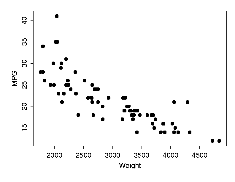 (Fig. 1)
Each dot in the figure provides information about the weight (x-axis, units: U.S. pounds) and fuel consumption (y-axis, units: miles per gallon) for one of 74 cars (data from 1979). Clearly weight and fuel consumption are linked, so that, in general, heavier cars use more fuel.
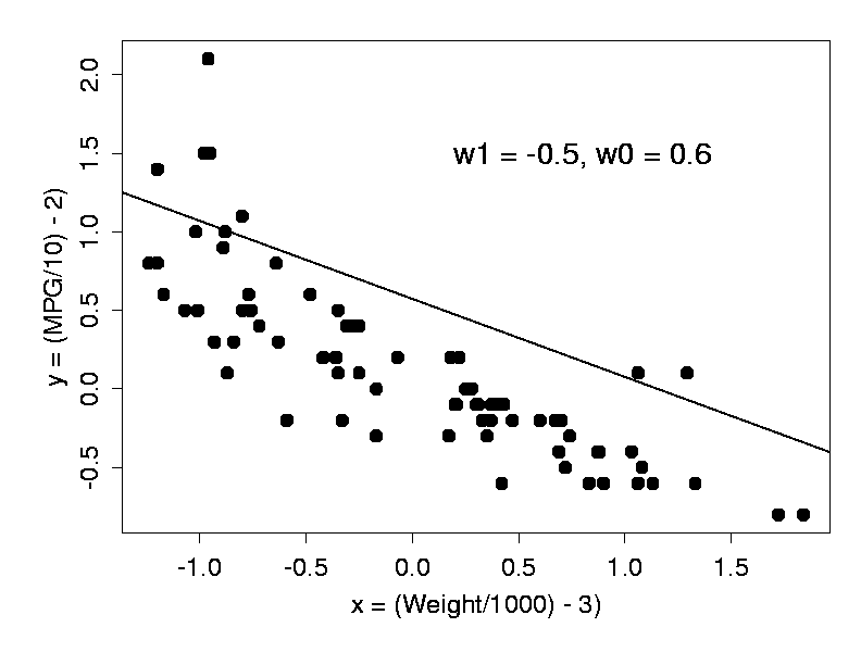
Now suppose we are given the weight of a 75th car, and asked to predict how much fuel it will use, based on the above data. Such questions can be answered by using amodel - a short mathematical description - of the data (see also optical illusions). The simplest useful model here is of the form
| y = w1 x + w0 | (1) |
This is a linear model: in an xy-plot, equation 1 describes a straight line with slope w1 and intercept w0 with the y-axis, as shown in Fig. 2. (Note that we have rescaled the coordinate axes - this does not change the problem in any fundamental way.)
How do we choose the two parameters w0 and w1 of our model? Clearly, any straight line drawn somehow through the data could be used as a predictor, but some lines will do a better job than others. The line in Fig. 2 is certainly not a good model: for most cars, it will predict too much fuel consumption for a given weight.
 (Fig. 2)
The Loss Function
In order to make precise what we mean by being a "good predictor", we define a loss (also called objective or error ) function E over the model parameters. A popular choice for E is the sum-squared error :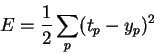 |
(2) |
In words, it is the sum over all points i in our data set of the squared difference between the target value ti (here: actual fuel consumption) and the model's prediction yi, calculated from the input value xi (here: weight of the car) by equation 1. For a linear model, the sum-sqaured error is a quadratic function of the model parameters. Figure 3 shows E for a range of values of w0 and w1. Figure 4 shows the same functions as a contour plot.
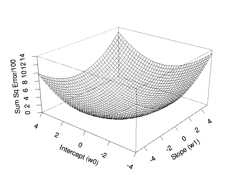 (Fig. 3)
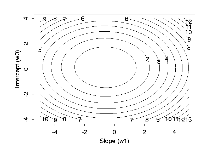 (Fig. 4)
Minimizing the Loss
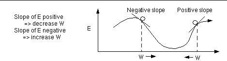
The loss function E provides us with an objective measure of predictive error for a specific choice of model parameters. We can thus restate our goal of finding the best (linear) model as finding the values for the model parameters that minimize E .For linear models, linear regression provides a direct way to compute these optimal model parameters. (See any statistics textbook for details.) However, this analytical approach does not generalize to nonlinear models (which we will get to by the end of this lecture). Even though the solution cannot be calculated explicitly in that case, the problem can still be solved by an iterative numerical technique called gradient descent. It works as follows:
- Choose some (random) initial values for the model parameters.
- Calculate the gradient G of the error function with respect to each model parameter.
- Change the model parameters so that we move a short distance in the direction of the greatest rate of decrease of the error, i.e., in the direction of -G.
- Repeat steps 2 and 3 until G gets close to zero.
 (Fig. 5)
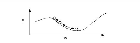
By repeating this over and over, we move "downhill" in E until we reach a minimum, where G = 0, so that no further progress is possible (Fig. 6).
 (Fig. 6)
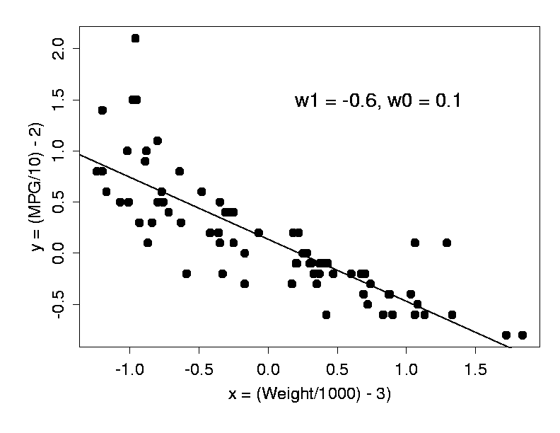
Fig. 7 shows the best linear model for our car data, found by this procedure.
 (Fig. 7)
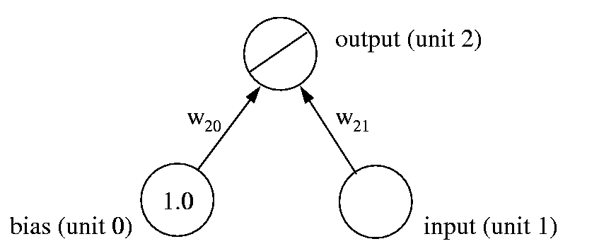
It's a neural network!
Our linear model of equation 1 can in fact be implemented by the simple neural network shown in Fig. 8. It consists of a bias unit, an input unit, and a linear output unit. The input unit makes external input x (here: the weight of a car) available to the network, while the bias unit always has a constant output of 1. The output unit computes the sum:|
|
(3)
|
It is easy to see that this is equivalent to equation 1, with w21 implementing the slope of the straight line, and w20 its intercept with the y-axis.
 (Fig. 8)
from: http://www.willamette.edu/~gorr/classes/cs449/linear1.html