classifier guided diffusion【公式加代码实战】Diffusion Models Beat GANs on Image Synthesis

一、前言

代码地址：https://github.com/openai/guided-diffusion
论文地址：https://arxiv.org/abs/2105.05233

二、训练的优化

参考https://blog.csdn.net/qq_45934285/article/details/129342977其实就是Improved DDPM的一些优化。

1. betas有两种类型"linear"和"cosine"其中cosine类型是优化的。
   
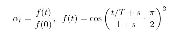
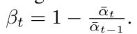
2. 学习方差，即上界和下界的一个插值
   
   学习方差的代码：

        model_output = model(x, self._scale_timesteps(t), **model_kwargs)
        # 得到方差和对数方差
        if self.model_var_type in [ModelVarType.LEARNED, ModelVarType.LEARNED_RANGE]:
            # 可学习的方差
            assert model_output.shape == (B, C * 2, *x.shape[2:])# 均值和方差二维
            model_output, model_var_values = th.split(model_output, C, dim=1)# 分割

            if self.model_var_type == ModelVarType.LEARNED:
                # 直接预测方差
                model_log_variance = model_var_values
                model_variance = th.exp(model_log_variance)
            else:
                # 预测方差插值的系数
                # 预测的范围是[-1,1]之间 公式14
                min_log = _extract_into_tensor(
                    self.posterior_log_variance_clipped, t, x.shape
                )
                max_log = _extract_into_tensor(np.log(self.betas), t, x.shape)
                # 对应两个方差的上下界
                # The model_var_values is [-1, 1] for [min_var, max_var].
                frac = (model_var_values + 1) / 2# 转换到[0,1]之间
                model_log_variance = frac * max_log + (1 - frac) * min_log
                model_variance = th.exp(model_log_variance)

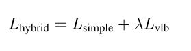
• 3.又因为由于Lsimple不依赖于 Σ θ(xt，t)，因此我们定义了一个新的混合目标函数:
  
• 4.当使用少于50个采样步骤时，我们采用DDIM这种采样方法，因为Nichol和Dhariwal [43] 发现它在这种情况下是有益的。
  加速采样。

5. 采用了重要性采样的策略。

1.评价指标（脑图）

三、架构优化

We explore the following architectural changes:

• Increasing depth versus width, holding model size relatively constant.
• Increasing the number of attention heads.
• Using attention at 32×32, 16×16, and 8×8 resolutions rather than only at 16×16.
• Using the BigGAN [5] residual block for upsampling and downsampling the activations,
  following [60].
• Rescaling residual connections with 1/根号2 , following [60, 27, 28].

然后是用了adaptive group normalization (AdaGN)
用time embedding和label embedding 去生成 $y_s$和$y_b$
$AdaGN(h,y)=y_{s}GroupNorm(h)+y_b$

其中h是在第一次卷积之后的残差块的中间激活。

四、条件生成

（1）一种straightforward的condition 扩散模型方法是将label信息进行embedding后加到time embedding中，但是效果不是很好。（Conditional）
代码：(具体代码在Unet中，就是将类条件加入embedding中)

#    :param num_classes: if specified (as an int), then this model will be
#        class-conditional with `num_classes` classes.
        if self.num_classes is not None:
            self.label_emb = nn.Embedding(num_classes, time_embed_dim)
#:param y: an [N] Tensor of labels, if class-conditional.
        assert (y is not None) == (
            self.num_classes is not None
        ), "must specify y if and only if the model is class-conditional"
        if self.num_classes is not None:
            assert y.shape == (x.shape[0],)
            emb = emb + self.label_emb(y)

所以本文加上了分类器指导的方法(并没有把上述的常规的condition生成方法丢弃)。具体的做法是在分类器中获取图片X的梯度，从而辅助模型进行采样生成图像。
下面介绍采样过程的具体细节（Guidance）

1.伪代码

Algorithm1是常规的DDPM采样过程，可见其变化的是$x_{t-1}$的采样过程的均值。（加了一个偏移量）
Algorithm2是DDIM的采样过程，其公式可以点开链接去看。

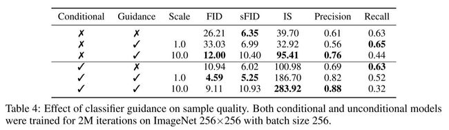
先看看效果：

2.公式推导

在证明之前有一些前置知识需要了解，否则推导过程很难理解。

1. 第一：（多元高斯分布的似然函数）
   
   这里最后一个公式等式的右边前两项是一个常数。也就是说以$\mu$为均值以$\sigma$为方差的==对数似然分布（log-likelihood function）==可以转为这种形式。看一个例子：(这里是一元的形式)
   
2. 第二个知识：多元分布协方差矩阵：即是对称矩阵，也是半正定矩阵。（其中对称矩阵性质要用到）

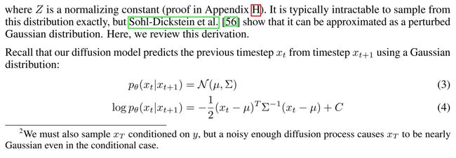
DDPM采样公式的证明

以下部分在附录H (P25-26)
一步一步来推导：

首先是给定的四个公式，在后面推导的时候会用到。

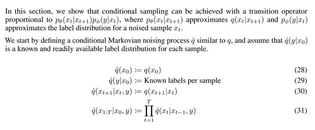
接下来分别证明q^的加噪条件分布、联合分布和边缘分布，在不加y条件的情况下,q ^与q的表现相同；并且进一步表明逆扩散条件分布也相同。

这证明了加噪过程q^不依赖于条件y，与q过程一样。

进一步证明了，q^与q的联合概率分布也一样。

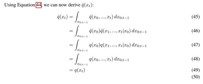
在第一部分给定了q^(y|x0)，那么q ^(y|xt)又具有什么样的性质呢？同时为了推导q ^(xt|xt+1,y)做铺垫：


从而得到最终的这个公式。
q(xt|xt+1)已经训练好了，只剩下q^(y|xt)这个分类器的训练。接下来看，如何从q ^(xt|xt+1,y)中逐步采样。

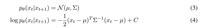
从上面的推导我们首先得到了这个公式：


公式（4）用到了上面讲的高斯概率分布转为对数似然分布的公式。

我们默认公式（5）的等式左边的公式是可微的，并且将其按泰勒展开公式在$x_t=\mu$处展开。这里的C1是因为将$x_t=\mu$其变为一个常数。


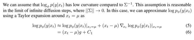
这里公式（7）到公式（8）是上面讲的，协方差矩阵是一个对称矩阵，转置等于其本身。
C2=C+c1

我们将公式（9）与公式（4）（3）进行对比，可以将对数似然概率转为高斯分布概率。
然后可以发现条件采样与非条件采样就相差一个均值的偏移在算法中我们在这个偏移项上乘了一个梯度尺度s

DDIM采样公式的证明

其为一个确定的抽样方法。

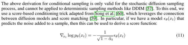
这是一个分数函数的表示形式

相当于将系数提出来了，然后就重新定义了一个噪声的采样公式。
然后给定了噪声，DDIM的采样公式$\sigma$为0
可以直接用均值去预测其分布。

到这里公式就推完了，接下来看看代码的实现：

五、代码实现部分

采样部分，
这里的cond_fn函数计算的是$s{\nabla }_{x_t}\log p_{\varphi }\left(y\mid x_t\right)$其中s 是 args.classifier_scale

    def cond_fn(x, t, y=None):#
        assert y is not None
        with th.enable_grad():
            x_in = x.detach().requires_grad_(True)
            logits = classifier(x_in, t)
            log_probs = F.log_softmax(logits, dim=-1)
            selected = log_probs[range(len(logits)), y.view(-1)]
            return th.autograd.grad(selected.sum(), x_in)[0] * args.classifier_scale

    def model_fn(x, t, y=None):#预测前一步的东西
        assert y is not None
        return model(x, t, y if args.class_cond else None)

    logger.log("sampling...")
    all_images = []
    all_labels = []
    while len(all_images) * args.batch_size < args.num_samples:
        model_kwargs = {}
        classes = th.randint(
            low=0, high=NUM_CLASSES, size=(args.batch_size,), device=dist_util.dev()
        )
        model_kwargs["y"] = classes
        sample_fn = (
            diffusion.p_sample_loop if not args.use_ddim else diffusion.ddim_sample_loop
        )
        sample = sample_fn(
            model_fn,
            (args.batch_size, 3, args.image_size, args.image_size),
            clip_denoised=args.clip_denoised,
            model_kwargs=model_kwargs,
            cond_fn=cond_fn,
            device=dist_util.dev(),
        )
        sample = ((sample + 1) * 127.5).clamp(0, 255).to(th.uint8)
        sample = sample.permute(0, 2, 3, 1)
        sample = sample.contiguous()

p_sample
guided_diffusion/gaussian_diffusion.py

    def p_sample(
        self,
        model,
        x,
        t,
        clip_denoised=True,
        denoised_fn=None,
        cond_fn=None,
        model_kwargs=None,
    ):
        """
        Sample x_{t-1} from the model at the given timestep.

        :param model: the model to sample from.
        :param x: the current tensor at x_{t-1}.
        :param t: the value of t, starting at 0 for the first diffusion step.
        :param clip_denoised: if True, clip the x_start prediction to [-1, 1].
        :param denoised_fn: if not None, a function which applies to the
            x_start prediction before it is used to sample.
        :param cond_fn: if not None, this is a gradient function that acts
                        similarly to the model.
        :param model_kwargs: if not None, a dict of extra keyword arguments to
            pass to the model. This can be used for conditioning.
        :return: a dict containing the following keys:
                 - 'sample': a random sample from the model.
                 - 'pred_xstart': a prediction of x_0.
        """
        out = self.p_mean_variance(
            model,
            x,
            t,
            clip_denoised=clip_denoised,
            denoised_fn=denoised_fn,
            model_kwargs=model_kwargs,
        )
        noise = th.randn_like(x)
        nonzero_mask = (
            (t != 0).float().view(-1, *([1] * (len(x.shape) - 1)))
        )  # no noise when t == 0
        if cond_fn is not None:# 修正均值
            out["mean"] = self.condition_mean(
                cond_fn, out, x, t, model_kwargs=model_kwargs
            )
        sample = out["mean"] + nonzero_mask * th.exp(0.5 * out["log_variance"]) * noise
        return {"sample": sample, "pred_xstart": out["pred_xstart"]}

可见多的代码是：

        if cond_fn is not None:# 修正均值
            out["mean"] = self.condition_mean(
                cond_fn, out, x, t, model_kwargs=model_kwargs
            )

可见这里就是最终的修正的均值：$\mu +s\Sigma {\nabla }_{x_t}\log p_{\varphi }\left(y\mid x_t\right)$

    def condition_mean(self, cond_fn, p_mean_var, x, t, model_kwargs=None):
        """
        Compute the mean for the previous step, given a function cond_fn that
        computes the gradient of a conditional log probability with respect to
        x. In particular, cond_fn computes grad(log(p(y|x))), and we want to
        condition on y.

        This uses the conditioning strategy from Sohl-Dickstein et al. (2015).
        """
        gradient = cond_fn(x, self._scale_timesteps(t), **model_kwargs)
        new_mean = (
            p_mean_var["mean"].float() + p_mean_var["variance"] * gradient.float()
        )
        return new_mean

ddim_sample
这是ddim的采样方法，关于这个在DDIM有介绍，不明白的请移步哦。这里只讲主要变换。

    def ddim_sample(
        self,
        model,
        x,
        t,
        clip_denoised=True,
        denoised_fn=None,
        cond_fn=None,
        model_kwargs=None,
        eta=0.0,
    ):
        """
        Sample x_{t-1} from the model using DDIM.

        Same usage as p_sample().
        """
        out = self.p_mean_variance(
            model,
            x,
            t,
            clip_denoised=clip_denoised,
            denoised_fn=denoised_fn,
            model_kwargs=model_kwargs,
        )
        if cond_fn is not None:
            out = self.condition_score(cond_fn, out, x, t, model_kwargs=model_kwargs)

        # Usually our model outputs epsilon, but we re-derive it
        # in case we used x_start or x_prev prediction.
        eps = self._predict_eps_from_xstart(x, t, out["pred_xstart"])

        alpha_bar = _extract_into_tensor(self.alphas_cumprod, t, x.shape)
        alpha_bar_prev = _extract_into_tensor(self.alphas_cumprod_prev, t, x.shape)
        sigma = (
            eta
            * th.sqrt((1 - alpha_bar_prev) / (1 - alpha_bar))
            * th.sqrt(1 - alpha_bar / alpha_bar_prev)
        )
        # Equation 12.
        noise = th.randn_like(x)
        mean_pred = (
            out["pred_xstart"] * th.sqrt(alpha_bar_prev)
            + th.sqrt(1 - alpha_bar_prev - sigma ** 2) * eps
        )
        nonzero_mask = (
            (t != 0).float().view(-1, *([1] * (len(x.shape) - 1)))
        )  # no noise when t == 0
        sample = mean_pred + nonzero_mask * sigma * noise
        return {"sample": sample, "pred_xstart": out["pred_xstart"]}

        if cond_fn is not None:
            out = self.condition_score(cond_fn, out, x, t, model_kwargs=model_kwargs)

condition_score

    def condition_score(self, cond_fn, p_mean_var, x, t, model_kwargs=None):
        """
        Compute what the p_mean_variance output would have been, should the
        model's score function be conditioned by cond_fn.

        See condition_mean() for details on cond_fn.

        Unlike condition_mean(), this instead uses the conditioning strategy
        from Song et al (2020).
        """
        alpha_bar = _extract_into_tensor(self.alphas_cumprod, t, x.shape)

        eps = self._predict_eps_from_xstart(x, t, p_mean_var["pred_xstart"])
        eps = eps - (1 - alpha_bar).sqrt() * cond_fn(
            x, self._scale_timesteps(t), **model_kwargs
        )

        out = p_mean_var.copy()
        out["pred_xstart"] = self._predict_xstart_from_eps(x, t, eps)
        out["mean"], _, _ = self.q_posterior_mean_variance(
            x_start=out["pred_xstart"], x_t=x, t=t
        )
        return out

这里用到的公式是：$\widehat{ϵ}\left(x_t\right):={ϵ}_{\theta }\left(x_t\right)-\sqrt{1-{\bar{\alpha }}_t}{\nabla }_{x_t}\log p_{\varphi }\left(y\mid x_t\right)$其中cond_fn返回值是$s{\nabla }_{x_t}\log p_{\varphi }\left(y\mid x_t\right)$
这里后面是用更新的噪声更新了一下模型的输出然后计算下一步：

这里$\eta$设为0.0故方差为0.

至此结束，感谢阅读^ - ^！
如果觉得有帮助的话，希望点赞收藏评论加关注支持一下吧。
你的支持是我创作的最大动力！！！

Reference：

1.https://www.bilibili.com/video/BV1m84y1e7hP/?spm_id_from=333.999.0.0&vd_source=5413f4289a5882463411525768a1ee27