python 中 任务 6.1 使用sklearn 转换器处理数据(划分训练集,测试集,PCA降维) 学习笔记1
文章目录
- 使用pandas进行数据预处理
- 任务 6.1 使用sklearn 转换器处理数据
-
- 6.1.1 加载datasets模块中的数据集
-
-
- datasets模块常用数据集的加载函数与解释如下表所示。
- 代码 6-1 加载breast_cancer 数据集
- 代码 6-2 sklearn 自带数据集内部消息获取
-
- 6.1.2 将数据集划分为训练集和测试集
-
- 常用划分方式
- K折交叉验证法
- 代码 6-3 使用train_test_split划分数据集
- 6.1.3 使用 sklearn 转换器进行数据预处理与降维
-
- sklearn 转换器三个方法
- sklearn转换器
- 代码 6-4 离差标准化
- 代码 6-5 对breast_cancer数据集PCA降维
- 6.1.4 任务实现
-
- 1.读取数据
- 代码 6-6 获取 sklearn 自带的boston数据集
- 2. 将数据集划分为训练集和测试集
- 6-7 使用train_test_split 划分boston数据集
- 6-8 使用stdScale.transform进行数据预处理
- 6-9 使用pcatransform 进行PCA降维
使用pandas进行数据预处理
任务 6.1 使用sklearn 转换器处理数据
6.1.1 加载datasets模块中的数据集
sklearn库的datasets模块集成了部分数据分析的经典数据集,可以使用这些数据集进行数据预处理,建模等操作,熟悉sklearn的数据处理流程和建模流程。
datasets模块常用数据集的加载函数与解释如下表所示。
%%html
<img src = './image/6-1-1.png',title = '11',width=100,height=100>
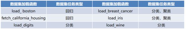
代码 6-1 加载breast_cancer 数据集
加载后的数据集可以视为一个字典,几乎所有的sklearn数据集均可以使用data,target,feature_names,DESCR分别获取数据集的数据,标签,特征名称和描述信息。
from sklearn.datasets import load_breast_cancer
cancer = load_breast_cancer()  ## 将数据集赋值给iris变量
print('breast_cancer数据集的长度为:',len(cancer))
print('breast_cancer数据集的类型为:',type(cancer))
breast_cancer数据集的长度为: 6
breast_cancer数据集的类型为:
代码 6-2 sklearn 自带数据集内部消息获取
cancer_data = cancer['data']
print('breast_cancer数据集的数据为:','\n',cancer_data)

cancer_target = cancer['target'] ## 取出数据集的标签
print('breast_cancer数据集的标签为:\n',cancer_target)

cancer_names = cancer['feature_names'] ## 取出数据集的特征名
print('breast_cancer数据集的特征名为:\n',cancer_names)

cancer_desc = cancer['DESCR'] ## 取出数据集的描述信息
print('breast_cancer数据集的描述信息为:\n',cancer_desc)
breast_cancer数据集的数据为:
 [[1.799e+01 1.038e+01 1.228e+02 ... 2.654e-01 4.601e-01 1.189e-01]
 [2.057e+01 1.777e+01 1.329e+02 ... 1.860e-01 2.750e-01 8.902e-02]
 [1.969e+01 2.125e+01 1.300e+02 ... 2.430e-01 3.613e-01 8.758e-02]
 ...
 [1.660e+01 2.808e+01 1.083e+02 ... 1.418e-01 2.218e-01 7.820e-02]
 [2.060e+01 2.933e+01 1.401e+02 ... 2.650e-01 4.087e-01 1.240e-01]
 [7.760e+00 2.454e+01 4.792e+01 ... 0.000e+00 2.871e-01 7.039e-02]]
breast_cancer数据集的标签为:
 [0 0 0 0 0 0 0 0 0 0 0 0 0 0 0 0 0 0 0 1 1 1 0 0 0 0 0 0 0 0 0 0 0 0 0 0 0
 1 0 0 0 0 0 0 0 0 1 0 1 1 1 1 1 0 0 1 0 0 1 1 1 1 0 1 0 0 1 1 1 1 0 1 0 0
 1 0 1 0 0 1 1 1 0 0 1 0 0 0 1 1 1 0 1 1 0 0 1 1 1 0 0 1 1 1 1 0 1 1 0 1 1
 1 1 1 1 1 1 0 0 0 1 0 0 1 1 1 0 0 1 0 1 0 0 1 0 0 1 1 0 1 1 0 1 1 1 1 0 1
 1 1 1 1 1 1 1 1 0 1 1 1 1 0 0 1 0 1 1 0 0 1 1 0 0 1 1 1 1 0 1 1 0 0 0 1 0
 1 0 1 1 1 0 1 1 0 0 1 0 0 0 0 1 0 0 0 1 0 1 0 1 1 0 1 0 0 0 0 1 1 0 0 1 1
 1 0 1 1 1 1 1 0 0 1 1 0 1 1 0 0 1 0 1 1 1 1 0 1 1 1 1 1 0 1 0 0 0 0 0 0 0
 0 0 0 0 0 0 0 1 1 1 1 1 1 0 1 0 1 1 0 1 1 0 1 0 0 1 1 1 1 1 1 1 1 1 1 1 1
 1 0 1 1 0 1 0 1 1 1 1 1 1 1 1 1 1 1 1 1 1 0 1 1 1 0 1 0 1 1 1 1 0 0 0 1 1
 1 1 0 1 0 1 0 1 1 1 0 1 1 1 1 1 1 1 0 0 0 1 1 1 1 1 1 1 1 1 1 1 0 0 1 0 0
 0 1 0 0 1 1 1 1 1 0 1 1 1 1 1 0 1 1 1 0 1 1 0 0 1 1 1 1 1 1 0 1 1 1 1 1 1
 1 0 1 1 1 1 1 0 1 1 0 1 1 1 1 1 1 1 1 1 1 1 1 0 1 0 0 1 0 1 1 1 1 1 0 1 1
 0 1 0 1 1 0 1 0 1 1 1 1 1 1 1 1 0 0 1 1 1 1 1 1 0 1 1 1 1 1 1 1 1 1 1 0 1
 1 1 1 1 1 1 0 1 0 1 1 0 1 1 1 1 1 0 0 1 0 1 0 1 1 1 1 1 0 1 1 0 1 0 1 0 0
 1 1 1 0 1 1 1 1 1 1 1 1 1 1 1 0 1 0 0 1 1 1 1 1 1 1 1 1 1 1 1 1 1 1 1 1 1
 1 1 1 1 1 1 1 0 0 0 0 0 0 1]
breast_cancer数据集的特征名为:
 ['mean radius' 'mean texture' 'mean perimeter' 'mean area'
 'mean smoothness' 'mean compactness' 'mean concavity'
 'mean concave points' 'mean symmetry' 'mean fractal dimension'
 'radius error' 'texture error' 'perimeter error' 'area error'
 'smoothness error' 'compactness error' 'concavity error'
 'concave points error' 'symmetry error' 'fractal dimension error'
 'worst radius' 'worst texture' 'worst perimeter' 'worst area'
 'worst smoothness' 'worst compactness' 'worst concavity'
 'worst concave points' 'worst symmetry' 'worst fractal dimension']
breast_cancer数据集的描述信息为:
 .. _breast_cancer_dataset:

Breast cancer wisconsin (diagnostic) dataset
--------------------------------------------

**Data Set Characteristics:**

    :Number of Instances: 569

    :Number of Attributes: 30 numeric, predictive attributes and the class

    :Attribute Information:
        - radius (mean of distances from center to points on the perimeter)
        - texture (standard deviation of gray-scale values)
        - perimeter
        - area
        - smoothness (local variation in radius lengths)
        - compactness (perimeter^2 / area - 1.0)
        - concavity (severity of concave portions of the contour)
        - concave points (number of concave portions of the contour)
        - symmetry
        - fractal dimension ("coastline approximation" - 1)

        The mean, standard error, and "worst" or largest (mean of the three
        largest values) of these features were computed for each image,
        resulting in 30 features.  For instance, field 3 is Mean Radius, field
        13 is Radius SE, field 23 is Worst Radius.

        - class:
                - WDBC-Malignant
                - WDBC-Benign

    :Summary Statistics:

    ===================================== ====== ======
                                           Min    Max
    ===================================== ====== ======
    radius (mean):                        6.981  28.11
    texture (mean):                       9.71   39.28
    perimeter (mean):                     43.79  188.5
    area (mean):                          143.5  2501.0
    smoothness (mean):                    0.053  0.163
    compactness (mean):                   0.019  0.345
    concavity (mean):                     0.0    0.427
    concave points (mean):                0.0    0.201
    symmetry (mean):                      0.106  0.304
    fractal dimension (mean):             0.05   0.097
    radius (standard error):              0.112  2.873
    texture (standard error):             0.36   4.885
    perimeter (standard error):           0.757  21.98
    area (standard error):                6.802  542.2
    smoothness (standard error):          0.002  0.031
    compactness (standard error):         0.002  0.135
    concavity (standard error):           0.0    0.396
    concave points (standard error):      0.0    0.053
    symmetry (standard error):            0.008  0.079
    fractal dimension (standard error):   0.001  0.03
    radius (worst):                       7.93   36.04
    texture (worst):                      12.02  49.54
    perimeter (worst):                    50.41  251.2
    area (worst):                         185.2  4254.0
    smoothness (worst):                   0.071  0.223
    compactness (worst):                  0.027  1.058
    concavity (worst):                    0.0    1.252
    concave points (worst):               0.0    0.291
    symmetry (worst):                     0.156  0.664
    fractal dimension (worst):            0.055  0.208
    ===================================== ====== ======

    :Missing Attribute Values: None

    :Class Distribution: 212 - Malignant, 357 - Benign

    :Creator:  Dr. William H. Wolberg, W. Nick Street, Olvi L. Mangasarian

    :Donor: Nick Street

    :Date: November, 1995

This is a copy of UCI ML Breast Cancer Wisconsin (Diagnostic) datasets.
https://goo.gl/U2Uwz2

Features are computed from a digitized image of a fine needle
aspirate (FNA) of a breast mass.  They describe
characteristics of the cell nuclei present in the image.

Separating plane described above was obtained using
Multisurface Method-Tree (MSM-T) [K. P. Bennett, "Decision Tree
Construction Via Linear Programming." Proceedings of the 4th
Midwest Artificial Intelligence and Cognitive Science Society,
pp. 97-101, 1992], a classification method which uses linear
programming to construct a decision tree.  Relevant features
were selected using an exhaustive search in the space of 1-4
features and 1-3 separating planes.

The actual linear program used to obtain the separating plane
in the 3-dimensional space is that described in:
[K. P. Bennett and O. L. Mangasarian: "Robust Linear
Programming Discrimination of Two Linearly Inseparable Sets",
Optimization Methods and Software 1, 1992, 23-34].

This database is also available through the UW CS ftp server:

ftp ftp.cs.wisc.edu
cd math-prog/cpo-dataset/machine-learn/WDBC/

.. topic:: References

   - W.N. Street, W.H. Wolberg and O.L. Mangasarian. Nuclear feature extraction
     for breast tumor diagnosis. IS&T/SPIE 1993 International Symposium on
     Electronic Imaging: Science and Technology, volume 1905, pages 861-870,
     San Jose, CA, 1993.
   - O.L. Mangasarian, W.N. Street and W.H. Wolberg. Breast cancer diagnosis and
     prognosis via linear programming. Operations Research, 43(4), pages 570-577,
     July-August 1995.
   - W.H. Wolberg, W.N. Street, and O.L. Mangasarian. Machine learning techniques
     to diagnose breast cancer from fine-needle aspirates. Cancer Letters 77 (1994)
     163-171.
6.1.2 将数据集划分为训练集和测试集
常用划分方式
在数据分析过程中,为了保证模型在实际系统中能够起到预期作用,一般需要将样本分成独立的三部分:
训练集(train set):用于估计模型。
验证集(validation set):用于确定网络结构或者控制模型复杂程度的参数。
测试集(test set):用于检验最优的模型的性能。
典型的划分方式是训练集占总样本的50%,而验证集和测试集各占25%。
K折交叉验证法
当数据总量较少的时候,使用上面的方法将数据划分为三部分就不合适了。
常用的方法是留少部分做测试集,然后对其余N个样本采用K折交叉验证法,基本步骤如下:
将样本打乱,均匀分成K份。
轮流选择其中K-1份做训练,剩余的一份做验证。
计算预测误差平方和,把K次的预测误差平方和的均值作为选择最优模型结构的依据。
代码 6-3 使用train_test_split划分数据集
print('原始数据集数据的形状为:',cancer_data.shape)
print('原始数据集标签的形状为:',cancer_target.shape)

from sklearn.model_selection import train_test_split
cancer_data_train,cancer_data_test,\
cancer_target_train,cancer_target_test = \
train_test_split(cancer_data,cancer_target,
                test_size = 0.2,random_state=42)
print('训练集数据的形状为:',cancer_data_train.shape)
print('训练集标签的形状为:',cancer_target_train.shape)
print('测试集数据的形状为:',cancer_data_test.shape)
print('测试集标签的形状为:',cancer_target_test.shape)
原始数据集数据的形状为: (569, 30)
原始数据集标签的形状为: (569,)
训练集数据的形状为: (455, 30)
训练集标签的形状为: (455,)
测试集数据的形状为: (114, 30)
测试集标签的形状为: (114,)
%%html
<img src = './image/6-1-2.png',title = '11',width=100,height=100>
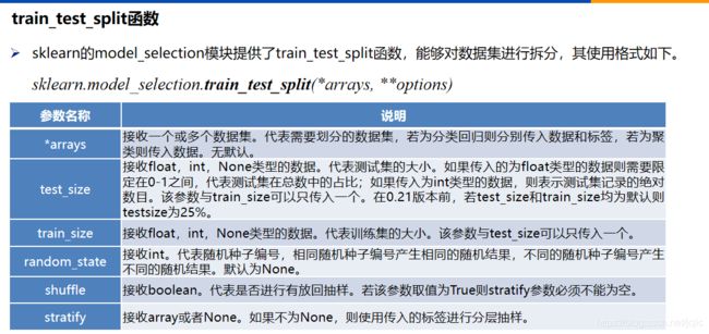
rain_test_split函数根据传入的数据,分别将传入的数据划分为训练集和测试集。
如果传入的是1组数据,那么生成的就是这一组数据随机划分后训练集和测试集,总共2组。如果传入的是2组数据,则生成的训练集和测试集分别2组,总共4组。
train_test_split是最常用的数据划分方法,在model_selection模块中还提供了其他数据集划分的函数,如PredefinedSplit,ShuffleSplit等。
6.1.3 使用 sklearn 转换器进行数据预处理与降维
sklearn 转换器三个方法
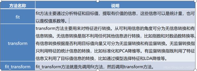
sklearn把相关的功能封装为转换器(transformer)。使用sklearn转换器能够实现对传入的NumPy数组进行标准化处理,归一化处理,二值化处理,PCA降维等操作。转换器主要包括三个方法:
%%html
<img src = './image/6-4.png',title = '11',width=100,height=100>
sklearn转换器
在数据分析过程中,各类特征处理相关的操作都需要对训练集和测试集分开操作,需要将训练集的操作规则,权重系数等应用到测试集中。
如果使用pandas,则应用至测试集的过程相对烦琐,使用sklearn转换器可以解决这一困扰。
代码 6-4 离差标准化
import numpy as np
from sklearn.preprocessing import MinMaxScaler
Scaler = MinMaxScaler().fit(cancer_data_train) ##生成规则
##将规则应用于训练集
cancer_trainScaler = Scaler.transform(cancer_data)
##将规则应用于测试集
cancer_testScaler = Scaler.transform(cancer_data_test)
print('离差标准化前训练集数据的最小值为:',np.min(cancer_data_train))
print('离差标准化后训练集数据的最小值为:',np.min(cancer_trainScaler))
print('离差标准化前训练集数据的最大值为:',np.max(cancer_data_train))
print('离差标准化后训练集数据的最大值为:',np.max(cancer_trainScaler))
print('离差标准化前测试集数据的最小值为:',np.min(cancer_data_test))
print('离差标准化后测试集数据的最小值为:',np.min(cancer_testScaler))
print('离差标准化前测试集数据的最大值为:',np.max(cancer_data_test))
print('离差标准化后测试集数据的最大值为:',np.max(cancer_testScaler))
离差标准化前训练集数据的最小值为: 0.0
离差标准化后训练集数据的最小值为: -0.057127602776294695
离差标准化前训练集数据的最大值为: 4254.0
离差标准化后训练集数据的最大值为: 1.3264399566986453
离差标准化前测试集数据的最小值为: 0.0
离差标准化后测试集数据的最小值为: -0.057127602776294695
离差标准化前测试集数据的最大值为: 3432.0
离差标准化后测试集数据的最大值为: 1.3264399566986453
%%html
<img src = './image/6-4.2.png',title = '11',width=100,height=100>
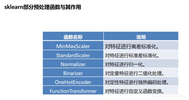
sklearn除了提供基本的特征变换函数外,还提供了降维算法,特征选择算法,这些算法的使用也是通过转换器的方式。
代码 6-5 对breast_cancer数据集PCA降维
%%html
<img src = './image/6-5.png',title = '11',width=700,height=100>
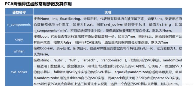
from sklearn.decomposition import PCA
pca_model = PCA(n_components=10).fit(cancer_trainScaler) ##生成规则
cancer_trainPca = pca_model.transform(cancer_trainScaler) ##将规则应用于训练集
cancer_testPca = pca_model.transform(cancer_testScaler) ##将规则应用于测试集
print('PCA降维前训练集数据的形状为:',cancer_trainScaler.shape)
print('PCA降维后训练集数据的形状为:',cancer_trainPca.shape)
print('PCA降维前测试集数据的形状为:',cancer_testScaler.shape)
print('PCA降维后测试集数据的形状为:',cancer_testPca.shape)
PCA降维前训练集数据的形状为: (569, 30)
PCA降维后训练集数据的形状为: (569, 10)
PCA降维前测试集数据的形状为: (114, 30)
PCA降维后测试集数据的形状为: (114, 10)
6.1.4 任务实现
1.读取数据
获取sklearn自带的boston数据集
代码 6-6 获取 sklearn 自带的boston数据集
from sklearn.datasets import load_boston
boston = load_boston()
boston_data = boston['data']
boston_target = boston['target']
boston_names = boston['feature_names']
print('boston数据集数据的形状为:',boston_data.shape)
print('boston数据集标签的形状为:',boston_target.shape)
print('boston数据集特征名的形状为:',boston_names.shape)
boston数据集数据的形状为: (506, 13)
boston数据集标签的形状为: (506,)
boston数据集特征名的形状为: (13,)
2. 将数据集划分为训练集和测试集
使用train_test_split划分boston数据集
6-7 使用train_test_split 划分boston数据集
from sklearn.model_selection import train_test_split
boston_data_train, boston_data_test, \
boston_target_train, boston_target_test = \
train_test_split(boston_data, boston_target,
    test_size=0.2, random_state=42)
print('训练集数据的形状为:',boston_data_train.shape)
print('训练集标签的形状为:',boston_target_train.shape)
print('测试集数据的形状为:',boston_data_test.shape)
print('测试集标签的形状为:',boston_target_test.shape)
训练集数据的形状为: (404, 13)
训练集标签的形状为: (404,)
测试集数据的形状为: (102, 13)
测试集标签的形状为: (102,)
6-8 使用stdScale.transform进行数据预处理
from sklearn.preprocessing import StandardScaler
stdScale = StandardScaler().fit(boston_data_train) ## 生成规则
## 将规则应用于训练集
boston_trainScaler = stdScale.transform(boston_data_train)
## 将规则应用于测试集
boston_testScaler = stdScale.transform(boston_data_test)
print('标准差标准化后训练集数据的方差为:',np.var(boston_trainScaler))
print('标准差标准化后训练集数据的均值为:',
    np.mean(boston_trainScaler))
print('标准差标准化后测试集数据的方差为:',np.var(boston_testScaler))
print('标准差标准化后测试集数据的均值为:',np.mean(boston_testScaler))
标准差标准化后训练集数据的方差为: 1.0
标准差标准化后训练集数据的均值为: 1.3637225393110834e-15
标准差标准化后测试集数据的方差为: 0.9474773930196593
标准差标准化后测试集数据的均值为: 0.030537934487192598
6-9 使用pcatransform 进行PCA降维
from sklearn.decomposition import PCA
pca = PCA(n_components=5).fit(boston_trainScaler) ## 生成规则
## 将规则应用于训练集
boston_trainPca = pca.transform(boston_trainScaler)
## 将规则应用于测试集
boston_testPca = pca.transform(boston_testScaler)
print('降维后boston数据集数据测试集的形状为:',boston_trainPca.shape)
print('降维后boston数据集数据训练集的形状为:',boston_testPca.shape)
降维后boston数据集数据测试集的形状为: (404, 5)
降维后boston数据集数据训练集的形状为: (102, 5)