- 英伟达Triton 推理服务详解
leo0308
基础知识机器人Triton人工智能
1.TritonInferenceServer简介TritonInferenceServer(简称Triton,原名NVIDIATensorRTInferenceServer)是英伟达推出的一个开源、高性能的推理服务器,专为AI模型的部署和推理服务而设计。它支持多种深度学习框架和硬件平台,能够帮助开发者和企业高效地将AI模型部署到生产环境中。Triton主要用于模型推理服务化,即将训练好的模型通过
- 「DR」沉渊/柳瑱
箫凌
站在黑暗的深处靠近光明的边缘刻铸最细腻的温情全世界只有不到3%的人微信搜索并且关注了箫凌你真是个特别的人策划:箫凌「fromOvertureStudio/角一文化」姓名:柳瑱生日:1993年12月4日星座:射手座Overture工作室/角一文化签约原创创作者作品:沉渊文案:柳瑱「fromOvertureStudio/角一文化」NOTE:其实我真不知道所谓创作构思要怎么写,那就罗列一些关于这个主题的
- PyTorch & TensorFlow速成复习:从基础语法到模型部署实战(附FPGA移植衔接)
阿牛的药铺
算法移植部署pytorchtensorflowfpga开发
PyTorch&TensorFlow速成复习:从基础语法到模型部署实战(附FPGA移植衔接)引言:为什么算法移植工程师必须掌握框架基础?针对光学类产品算法FPGA移植岗位需求(如可见光/红外图像处理),深度学习框架是算法落地的"桥梁"——既要用PyTorch/TensorFlow验证算法可行性,又要将训练好的模型(如CNN、目标检测)转换为FPGA可部署的格式(ONNX、TFLite)。本文采用"
- 边缘人工智能与医疗AI融合发展路径:技术融合与应用前景(上)
Allen_Lyb
数智化医院2025人工智能健康医疗算法
引言人工智能技术正以前所未有的速度改变着医疗保健领域,从辅助诊断到个性化治疗,AI应用的广度和深度不断拓展。在这一浪潮中,边缘人工智能(EdgeAI)作为一种新兴技术范式,正成为推动医疗AI创新的关键力量。边缘AI区别于传统的云计算模式,它将数据处理和AI模型部署在数据源头附近,实现快速响应和隐私保护。这种特性使其在医疗保健领域具有独特优势,特别是在实时监测、紧急响应和患者隐私保护等方面。边缘AI
- 一文读懂 Sigmoid 与 Hard Sigmoid 激活函数:从原理到量化部署
算法自动驾驶
在神经网络训练与部署中,激活函数扮演着关键角色,不仅影响模型训练过程,也直接决定了模型部署到实际设备后的性能表现。本文将介绍两种常用激活函数:Sigmoid和HardSigmoid,全面对比它们的原理、优缺点、应用场景,并提供实际代码示例,帮助你更好地理解与使用它们,尤其是在量化和嵌入式设备部署场景中。一、Sigmoid与HardSigmoid简介1.1Sigmoid激活函数介绍Sigmoid激活
- 【机器学习笔记 Ⅱ】10 完整周期
机器学习的完整生命周期(End-to-EndPipeline)机器学习的完整周期涵盖从问题定义到模型部署的全过程,以下是系统化的步骤分解和关键要点:1.问题定义(ProblemDefinition)目标:明确业务需求与机器学习任务的匹配性。关键问题:这是分类、回归、聚类还是强化学习问题?成功的标准是什么?(如准确率>90%、降低10%成本)输出:项目目标文档(含评估指标)。2.数据收集(DataC
- 超详细yolov8/11-segment实例分割全流程概述:配置环境、数据标注、训练、验证/预测、onnx部署(c++/python)详解
因为yolo的检测/分割/姿态/旋转/分类模型的环境配置、训练、推理预测等命令非常类似,这里不再详细叙述,主要参考**【YOLOv8/11-detect目标检测全流程教程】**,下面有相关链接,这里主要针对数据标注、格式转换、模型部署等不同细节部分;【YOLOv8/11-detect目标检测全流程教程】超详细yolo8/11-detect目标检测全流程概述:配置环境、数据标注、训练、验证/预测、o
- 使用TVM编译部署DarkNet模型:YOLO-V2和YOLO-V3实战指南
周情津Raymond
使用TVM编译部署DarkNet模型:YOLO-V2和YOLO-V3实战指南tvm-cnTVMDocumentationinChineseSimplified/TVM中文文档项目地址:https://gitcode.com/gh_mirrors/tv/tvm-cn前言在深度学习模型部署领域,TVM作为一个高效的深度学习编译器栈,能够将训练好的模型优化并部署到各种硬件平台上。本文将详细介绍如何使用T
- Ollama-python:调用大模型服务实现代码自动补全,提升编程开发效率!
Ollama是一个优秀的本地部署与管理大模型的框架。通过Ollama,我们可以在本地部署、定制自己的大模型服务。大模型部署在本地后,我们可以有哪些应用呢?本文介绍如何通过Ollama的pythonsdk,调用本地部署的大模型服务,对我们的代码进行自动补全,提升日常的编程开发效率。安装Ollama及其pythonsdk在https://ollama.com/download下载Ollama安装程序并
- 文心4.5开源模型部署实践
skywalk8163
人工智能文心人工智能文心大模型开源大模型文心开源
文心4.5开源模型部署实践使用fastdeploy本地部署执行命令:python-mfastdeploy.entrypoints.openai.api_server\ --modelbaidu/ERNIE-4.5-21B-A3B-Paddle\ --port8180\ --metrics-port8181\ --engine-worker-queue-port8182\ --max-model-l
- 重构企业智能服务:大模型部署背后的战略与落地实践
慌ZHANG
人工智能人工智能
个人主页:慌ZHANG-CSDN博客期待您的关注一、引言:从“能用”到“可用”的时代跃迁过去一年中,大语言模型(LLMs)实现了从实验室“黑科技”到企业场景“生产力”的巨大跃迁。无论是通用问答、客户支持、文本生成、知识库问询,还是代码辅助、财报分析,大模型的边界已快速渗透到各行各业。然而,许多企业在试图将ChatGPT或DeepSeek等模型引入自己的业务系统时却发现:在线服务存在数据泄露风险;响
- mlflow案例
以下内容主要是翻译mlflow官方文档的一个教程。4.教程和示例4.1训练、服务和评估线性回归模型地址:Tutorial—MLflow2.4.1documentation本教程展示了如何使用MLflow端到端执行以下操作:(1)训练线性回归模型(2)将训练模型的代码打包为可重复使用和可复制的模型格式(3)将模型部署到一个简单的HTTP服务器中,使您能够对预测进行评分本教程使用的数据集将根据葡萄酒的
- pythonflow_MLflow系列1:MLflow入门教程(Python)
weixin_39872334
pythonflow
这篇教程展示了如何:训练一个线性回归模型将训练代码打包成一个可复用可复现的模型格式将模型部署成一个简单的HTTP服务用于进行预测这篇教程使用的数据来自UCI的红酒质量数据集,主要用于根据红酒的PH值,酸度,残糖量等指标来评估红酒的质量。我们会用到什么?安装MLflow和scikit-learn,推荐两种安装方式:安装MLflow及其依赖:pipinstallmlflow[extras]分别安装ML
- BAAI/BGE-VL多模态模型部署、原理、代码详解(实现图像文本混合检索),包含BEG-VL多模态模型的本地部署详细步骤及代码原理解析
令令小宁
python语言模型自然语言处理nlp人工智能
本文包含BGE-VL多模态模型的本地部署详细步骤及代码原理解析文章目录前言一、模型下载二、计算流程解析1.BGE-VL-base/Large2.BGE-VL-MLLM-s1/s2三、总结前言提示:这里可以添加本文要记录的大概内容:包含四个模型及数据集,数据集未开源,四个模型可以分别下载:其中,BGE-VL-base/Large是基于CLIP训练的模型,BGE-VL-MLLM-S1/S2是基于LLM
- 【模型部署】如何在Linux中通过脚本文件部署模型
满怀1015
人工智能linux网络人工只能模型部署
在Linux中,你可以将部署命令保存为可执行脚本文件,并通过终端直接调用。以下是几种常见且实用的方法:方法1:Shell脚本(推荐)步骤创建一个.sh文件(例如start_vllm.sh):#!/bin/bashCUDA_VISIBLE_DEVICES=7\python-mvllm.entrypoints.openai.api_server\--served-model-nameQwen2-7B-
- Spring Boot + ONNX Runtime模型部署
文章目录前言一、模型导出二、Java推理引擎选型三、SpringBoot实战3.1核心架构3.2分层架构详细实现1.Controller层-请求入口2.Service层-核心业务流程3.关键组件深度优化四、云原生部署:Docker+Kubernetes总结前言在AI浪潮席卷全球的今天,Java工程师如何守住后端主战场?模型部署正是Java工程师融入AI领域的方向。为什么Java工程师必须掌握模型部
- onnx模型部署 python_深度学习模型转换与部署那些事(含ONNX格式详细分析)
weixin_39759270
onnx模型部署python
背景深度学习模型在训练完成之后,部署并应用在生产环境的这一步至关重要,毕竟训练出来的模型不能只接受一些公开数据集和榜单的检验,还需要在真正的业务场景下创造价值,不能只是为了PR而躺在实验机器上在现有条件下,一般涉及到模型的部署就要涉及到模型的转换,而转换的过程也是随着对应平台的不同而不同,一般工程师接触到的平台分为GPU云平台、手机和其他嵌入式设备对于GPU云平台来说,在上面部署本应该是最轻松的事
- vLLM调度部署Qwen3
你好,此用户已存在
人工智能linux大模型
vLLM介绍在之前的文章中,我们介绍了如何使用ollama部署qwen3,一般而言,ollama适合个人部署使用,在面对企业级的模型部署时,一般更建议使用vLLMvLLM(高效大语言模型推理库)是一个专为大语言模型(LLMs)优化推理速度的开源框架,由斯坦福大学系统研究组开发。其核心目标是通过创新的软件和算法设计,大幅提升LLM在生成文本时的吞吐量和效率,尤其适用于处理高并发的推理请求。从各种基准
- 如何构建AI原生应用领域的高效SaaS架构
AI原生应用开发
AI-native架构ai
如何构建AI原生应用领域的高效SaaS架构关键词:AI原生应用、SaaS架构、微服务、容器化、机器学习模型部署、自动扩展、多租户隔离摘要:本文深入探讨如何构建面向AI原生应用的高效SaaS架构。我们将从基础概念出发,逐步解析AISaaS架构的核心组件、设计原则和最佳实践,并通过实际案例展示如何实现高性能、可扩展的AI服务交付平台。文章将涵盖从基础设施选择到模型部署,从多租户隔离到自动扩展的全方位技
- 使用 Xinference 命令行工具(xinference launch)部署 Nanonets-OCR-s
没刮胡子
Linux服务器技术人工智能AI软件开发技术实战专栏ocr
使用Xinference命令行工具(xinferencelaunch)部署Nanonets-OCR-s一、核心优势与适用场景通过xinferencelaunch命令可直接在命令行完成模型部署,无需编写Python代码,适合快速验证或生产环境批量部署。二、部署步骤:从命令行启动模型1.确认环境与依赖已安装Xinference:pipinstall"xinference[all]"GPU显存≥9GB(
- AingDesk开源免费的本地 AI 模型管理工具(搭建和调用MCP)
没刮胡子
Linux服务器技术软件开发技术实战专栏人工智能AI开源人工智能AI助手mcpsse知识库智能体
说明AingDesk是一款开源免费的本地AI模型管理工具,旨在简化AI模型部署流程并提升用户体验。AingDesk支持本地AI模型及API+知识库搭建。支持知识库、模型API、分享、联网搜索、智能体。✨产品亮点跨平台支持客户端支持Windows、macOS,服务端可通过Docker部署高效下载与网络优化自动选择最优下载线路,支持断点续传,提升大模型部署速度兼容OpenAIAPI格式,方便第三方模型
- 解密大模型全栈开发:从搭建环境到实战案例,一站式攻略
海棠AI实验室
“智元启示录“-AI发展的深度思考与未来展望人工智能大模型全栈开发
目录大模型基础概念什么是大模型?大模型的发展历程大模型的类型大模型全栈开发环境搭建硬件需求软件环境配置云服务选择大模型应用开发流程模型选择策略提示工程(PromptEngineering)模型微调(Fine-tuning)参数高效微调(PEFT)大模型应用架构设计基本应用架构RAG(检索增强生成)系统Agent系统设计大模型应用部署与优化模型部署选项模型优化技术性能监控与调优大模型应用实战案例智能
- PyTorch教程:LSTM语言模型的动态量化技术解析
怀灏其Prudent
PyTorch教程:LSTM语言模型的动态量化技术解析tutorialsPyTorchtutorials.项目地址:https://gitcode.com/gh_mirrors/tuto/tutorials前言在深度学习模型部署过程中,模型大小和推理速度是两个至关重要的考量因素。PyTorch提供的动态量化技术能够在不显著影响模型准确率的前提下,有效减小模型体积并提升推理速度。本文将深入解析如何对
- 从实验到生产:DeepSeek大模型工程化部署的关键步骤与风险控制
一ge科研小菜菜
人工智能人工智能
个人主页:一ge科研小菜鸡-CSDN博客期待您的关注一、引言:大模型部署迈入“工程化时代”随着DeepSeek等开源大语言模型(LLM)的发展,大模型不再是AI实验室的专属工具,越来越多的企业正尝试将其纳入业务生产系统,应用于客服问答、合同审查、数据分析、自动写作等场景。但模型的能力≠可用的系统。从模型下载到模型上线,中间隔着“部署的鸿沟”:资源配置、服务稳定性、响应效率、安全控制、上线合规……一
- DeepSeek 部署中的常见问题及解决方案:从环境配置到性能优化的全流程指南
慌ZHANG
人工智能人工智能
个人主页:慌ZHANG-CSDN博客期待您的关注一、引言:大模型部署的现实挑战随着大模型技术的发展,以DeepSeek为代表的开源中文大模型,逐渐成为企业与开发者探索私有化部署、垂直微调、模型服务化的重要选择。然而,模型部署的过程并非“一键启动”那么简单。从环境依赖、资源限制,到推理性能和服务稳定性,开发者往往会遇到一系列“踩坑点”。本文将系统梳理DeepSeek模型在部署过程中的典型问题与实践经
- MI300X vs H100:DeepSeek 部署在哪个 GPU 上性价比最高?
卓普云
技术科普AIGC人工智能DeepseekH100MI300x
随着大模型部署和推理变得越来越普及,开发者和企业对GPU的选择也越来越挑剔。特别是像DeepSeek这样的开源模型家族,从轻量级的6.7B,到动辄上百亿甚至数百亿参数的超大模型,背后对算力和显存的要求各不相同。最近,一则重磅消息在AI圈引起了轩然大波:连AI巨头OpenAI也在探索并计划使用AMDInstinctMI300xGPU!这无疑是对AMD这款高性能GPU的巨大认可,也预示着它将在AI算力
- 【软件系统架构】系列四:嵌入式软件-NPU(神经网络处理器)系统及模板
目录一、什么是NPU?二、NPU与CPU/GPU/DSP对比三、NPU的工作原理核心结构:数据流架构:四、NPU芯片架构(简化图)五、NPU的优势六、NPU应用场景视觉识别语音识别自动驾驶智能监控AIoT设备七、主流NPU芯片/架构实例八、开发者工具生态(通用)九、NPU集成建议(嵌入式开发场景)十、NPU芯片选型对比+模型部署流程+嵌入式工程模板1.主流NPU芯片选型对比表2.模型部署流程(以T
- 【高频考点精讲】前端AI集成实战:从TensorFlow.js到模型部署
全栈老李技术面试
前端高频考点精讲前端javascripthtmlcss面试题reactvue
前端AI集成实战:从TensorFlow.js到模型部署作者:全栈老李更新时间:2025年5月适合人群:前端初学者、进阶开发者版权:本文由全栈老李原创,转载请注明出处。今天咱们聊聊前端工程师如何玩转AI——没错,用JavaScript就能搞机器学习!我是全栈老李,一个喜欢把复杂技术讲简单的实战派。最近发现不少前端同学对AI既好奇又害怕,其实真没想象中那么难,跟着老李走,30分钟让你亲手部署第一
- 【机器学习的五大核心步骤】从零构建一个智能系统
目录一、数据处理:一切从“数据”开始✅常见数据源✅关键任务二、特征工程:从“数据”中提取“洞察”✅常用方法✅高阶技巧三、建立模型:从“算法”到“智能”✅模型类型✅常见算法✅模型训练四、评估迭代:没有反馈,就没有智能✅常用评估指标✅迭代优化方法五、上线应用与持续优化:从“实验室”到“真实世界”✅模型部署方式✅持续优化总结:看懂全流程!延伸阅读推荐作者:一叶轻舟|AI应用开发者&技术博主日期:2025
- C4.5算法深度解析:决策树进化的里程碑
大千AI助手
算法决策树机器学习C4.5Python人工智能AI
C4.5是机器学习史上最经典的算法之一,由ID3之父RossQuinlan在1993年提出。作为ID3的革命性升级,它不仅解决了前代的核心缺陷,更开创了连续特征处理和剪枝技术的先河,成为现代决策树的奠基之作。本文由「大千AI助手」原创发布,专注用真话讲AI,回归技术本质。拒绝神话或妖魔化。搜索「大千AI助手」关注我,一起撕掉过度包装,学习真实的AI技术!往期文章推荐:20.用Mermaid代码画E
- HQL之投影查询
归来朝歌
HQLHibernate查询语句投影查询
在HQL查询中,常常面临这样一个场景,对于多表查询,是要将一个表的对象查出来还是要只需要每个表中的几个字段,最后放在一起显示?
针对上面的场景,如果需要将一个对象查出来:
HQL语句写“from 对象”即可
Session session = HibernateUtil.openSession();
- Spring整合redis
bylijinnan
redis
pom.xml
<dependencies>
<!-- Spring Data - Redis Library -->
<dependency>
<groupId>org.springframework.data</groupId>
<artifactId>spring-data-redi
- org.hibernate.NonUniqueResultException: query did not return a unique result: 2
0624chenhong
Hibernate
参考:http://blog.csdn.net/qingfeilee/article/details/7052736
org.hibernate.NonUniqueResultException: query did not return a unique result: 2
在项目中出现了org.hiber
- android动画效果
不懂事的小屁孩
android动画
前几天弄alertdialog和popupwindow的时候,用到了android的动画效果,今天专门研究了一下关于android的动画效果,列出来,方便以后使用。
Android 平台提供了两类动画。 一类是Tween动画,就是对场景里的对象不断的进行图像变化来产生动画效果(旋转、平移、放缩和渐变)。
第二类就是 Frame动画,即顺序的播放事先做好的图像,与gif图片原理类似。
- js delete 删除机理以及它的内存泄露问题的解决方案
换个号韩国红果果
JavaScript
delete删除属性时只是解除了属性与对象的绑定,故当属性值为一个对象时,删除时会造成内存泄露 (其实还未删除)
举例:
var person={name:{firstname:'bob'}}
var p=person.name
delete person.name
p.firstname -->'bob'
// 依然可以访问p.firstname,存在内存泄露
- Oracle将零干预分析加入网络即服务计划
蓝儿唯美
oracle
由Oracle通信技术部门主导的演示项目并没有在本月较早前法国南斯举行的行业集团TM论坛大会中获得嘉奖。但是,Oracle通信官员解雇致力于打造一个支持零干预分配和编制功能的网络即服务(NaaS)平台,帮助企业以更灵活和更适合云的方式实现通信服务提供商(CSP)的连接产品。这个Oracle主导的项目属于TM Forum Live!活动上展示的Catalyst计划的19个项目之一。Catalyst计
- spring学习——springmvc(二)
a-john
springMVC
Spring MVC提供了非常方便的文件上传功能。
1,配置Spring支持文件上传:
DispatcherServlet本身并不知道如何处理multipart的表单数据,需要一个multipart解析器把POST请求的multipart数据中抽取出来,这样DispatcherServlet就能将其传递给我们的控制器了。为了在Spring中注册multipart解析器,需要声明一个实现了Mul
- POJ-2828-Buy Tickets
aijuans
ACM_POJ
POJ-2828-Buy Tickets
http://poj.org/problem?id=2828
线段树,逆序插入
#include<iostream>#include<cstdio>#include<cstring>#include<cstdlib>using namespace std;#define N 200010struct
- Java Ant build.xml详解
asia007
build.xml
1,什么是antant是构建工具2,什么是构建概念到处可查到,形象来说,你要把代码从某个地方拿来,编译,再拷贝到某个地方去等等操作,当然不仅与此,但是主要用来干这个3,ant的好处跨平台 --因为ant是使用java实现的,所以它跨平台使用简单--与ant的兄弟make比起来语法清晰--同样是和make相比功能强大--ant能做的事情很多,可能你用了很久,你仍然不知道它能有
- android按钮监听器的四种技术
百合不是茶
androidxml配置监听器实现接口
android开发中经常会用到各种各样的监听器,android监听器的写法与java又有不同的地方;
1,activity中使用内部类实现接口 ,创建内部类实例 使用add方法 与java类似
创建监听器的实例
myLis lis = new myLis();
使用add方法给按钮添加监听器
- 软件架构师不等同于资深程序员
bijian1013
程序员架构师架构设计
本文的作者Armel Nene是ETAPIX Global公司的首席架构师,他居住在伦敦,他参与过的开源项目包括 Apache Lucene,,Apache Nutch, Liferay 和 Pentaho等。
如今很多的公司
- TeamForge Wiki Syntax & CollabNet User Information Center
sunjing
TeamForgeHow doAttachementAnchorWiki Syntax
the CollabNet user information center http://help.collab.net/
How do I create a new Wiki page?
A CollabNet TeamForge project can have any number of Wiki pages. All Wiki pages are linked, and
- 【Redis四】Redis数据类型
bit1129
redis
概述
Redis是一个高性能的数据结构服务器,称之为数据结构服务器的原因是,它提供了丰富的数据类型以满足不同的应用场景,本文对Redis的数据类型以及对这些类型可能的操作进行总结。
Redis常用的数据类型包括string、set、list、hash以及sorted set.Redis本身是K/V系统,这里的数据类型指的是value的类型,而不是key的类型,key的类型只有一种即string
- SSH2整合-附源码
白糖_
eclipsespringtomcatHibernateGoogle
今天用eclipse终于整合出了struts2+hibernate+spring框架。
我创建的是tomcat项目,需要有tomcat插件。导入项目以后,鼠标右键选择属性,然后再找到“tomcat”项,勾选一下“Is a tomcat project”即可。具体方法见源码里的jsp图片,sql也在源码里。
补充1:项目中部分jar包不是最新版的,可能导
- [转]开源项目代码的学习方法
braveCS
学习方法
转自:
http://blog.sina.com.cn/s/blog_693458530100lk5m.html
http://www.cnblogs.com/west-link/archive/2011/06/07/2074466.html
1)阅读features。以此来搞清楚该项目有哪些特性2)思考。想想如果自己来做有这些features的项目该如何构架3)下载并安装d
- 编程之美-子数组的最大和(二维)
bylijinnan
编程之美
package beautyOfCoding;
import java.util.Arrays;
import java.util.Random;
public class MaxSubArraySum2 {
/**
* 编程之美 子数组之和的最大值(二维)
*/
private static final int ROW = 5;
private stat
- 读书笔记-3
chengxuyuancsdn
jquery笔记resultMap配置ibatis一对多配置
1、resultMap配置
2、ibatis一对多配置
3、jquery笔记
1、resultMap配置
当<select resultMap="topic_data">
<resultMap id="topic_data">必须一一对应。
(1)<resultMap class="tblTopic&q
- [物理与天文]物理学新进展
comsci
如果我们必须获得某种地球上没有的矿石,才能够进行某些能量输出装置的设计和建造,而要获得这种矿石,又必须首先进行深空探测,而要进行深空探测,又必须获得这种能量输出装置,这个矛盾的循环,会导致地球联盟在与宇宙文明建立关系的时候,陷入困境
怎么办呢?
- Oracle 11g新特性:Automatic Diagnostic Repository
daizj
oracleADR
Oracle Database 11g的FDI(Fault Diagnosability Infrastructure)是自动化诊断方面的又一增强。
FDI的一个关键组件是自动诊断库(Automatic Diagnostic Repository-ADR)。
在oracle 11g中,alert文件的信息是以xml的文件格式存在的,另外提供了普通文本格式的alert文件。
这两份log文
- 简单排序:选择排序
dieslrae
选择排序
public void selectSort(int[] array){
int select;
for(int i=0;i<array.length;i++){
select = i;
for(int k=i+1;k<array.leng
- C语言学习六指针的经典程序,互换两个数字
dcj3sjt126com
c
示例程序,swap_1和swap_2都是错误的,推理从1开始推到2,2没完成,推到3就完成了
# include <stdio.h>
void swap_1(int, int);
void swap_2(int *, int *);
void swap_3(int *, int *);
int main(void)
{
int a = 3;
int b =
- php 5.4中php-fpm 的重启、终止操作命令
dcj3sjt126com
PHP
php 5.4中php-fpm 的重启、终止操作命令:
查看php运行目录命令:which php/usr/bin/php
查看php-fpm进程数:ps aux | grep -c php-fpm
查看运行内存/usr/bin/php -i|grep mem
重启php-fpm/etc/init.d/php-fpm restart
在phpinfo()输出内容可以看到php
- 线程同步工具类
shuizhaosi888
同步工具类
同步工具类包括信号量(Semaphore)、栅栏(barrier)、闭锁(CountDownLatch)
闭锁(CountDownLatch)
public class RunMain {
public long timeTasks(int nThreads, final Runnable task) throws InterruptedException {
fin
- bleeding edge是什么意思
haojinghua
DI
不止一次,看到很多讲技术的文章里面出现过这个词语。今天终于弄懂了——通过朋友给的浏览软件,上了wiki。
我再一次感到,没有辞典能像WiKi一样,给出这样体贴人心、一清二楚的解释了。为了表达我对WiKi的喜爱,只好在此一一中英对照,给大家上次课。
In computer science, bleeding edge is a term that
- c中实现utf8和gbk的互转
jimmee
ciconvutf8&gbk编码
#include <iconv.h>
#include <stdlib.h>
#include <stdio.h>
#include <unistd.h>
#include <fcntl.h>
#include <string.h>
#include <sys/stat.h>
int code_c
- 大型分布式网站架构设计与实践
lilin530
应用服务器搜索引擎
1.大型网站软件系统的特点?
a.高并发,大流量。
b.高可用。
c.海量数据。
d.用户分布广泛,网络情况复杂。
e.安全环境恶劣。
f.需求快速变更,发布频繁。
g.渐进式发展。
2.大型网站架构演化发展历程?
a.初始阶段的网站架构。
应用程序,数据库,文件等所有的资源都在一台服务器上。
b.应用服务器和数据服务器分离。
c.使用缓存改善网站性能。
d.使用应用
- 在代码中获取Android theme中的attr属性值
OliveExcel
androidtheme
Android的Theme是由各种attr组合而成, 每个attr对应了这个属性的一个引用, 这个引用又可以是各种东西.
在某些情况下, 我们需要获取非自定义的主题下某个属性的内容 (比如拿到系统默认的配色colorAccent), 操作方式举例一则:
int defaultColor = 0xFF000000;
int[] attrsArray = { andorid.r.
- 基于Zookeeper的分布式共享锁
roadrunners
zookeeper分布式共享锁
首先,说说我们的场景,订单服务是做成集群的,当两个以上结点同时收到一个相同订单的创建指令,这时并发就产生了,系统就会重复创建订单。等等......场景。这时,分布式共享锁就闪亮登场了。
共享锁在同一个进程中是很容易实现的,但在跨进程或者在不同Server之间就不好实现了。Zookeeper就很容易实现。具体的实现原理官网和其它网站也有翻译,这里就不在赘述了。
官
- 两个容易被忽略的MySQL知识
tomcat_oracle
mysql
1、varchar(5)可以存储多少个汉字,多少个字母数字? 相信有好多人应该跟我一样,对这个已经很熟悉了,根据经验我们能很快的做出决定,比如说用varchar(200)去存储url等等,但是,即使你用了很多次也很熟悉了,也有可能对上面的问题做出错误的回答。 这个问题我查了好多资料,有的人说是可以存储5个字符,2.5个汉字(每个汉字占用两个字节的话),有的人说这个要区分版本,5.0
- zoj 3827 Information Entropy(水题)
阿尔萨斯
format
题目链接:zoj 3827 Information Entropy
题目大意:三种底,计算和。
解题思路:调用库函数就可以直接算了,不过要注意Pi = 0的时候,不过它题目里居然也讲了。。。limp→0+plogb(p)=0,因为p是logp的高阶。
#include <cstdio>
#include <cstring>
#include <cmath&
 其中, E E E 为损失函数, w w w 为权重向量, H = ∂ 2 E / ∂ w 2 H=\partial^2E/\partial w^2 H=∂2E/∂w2 为 Hessian matrix. 类似于 OBD,为了简化上式,作者假设剪枝前模型权重已位于局部最小点从而省略第一项,假设目标函数近似二次函数从而省略第三项,但需要注意的是,不同于 OBD,这里作者并没有使用 “diagonal” approximation,不假设 H H H 为对角矩阵。这样上式就简化为了
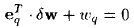 其中, e q e_q eq 为对应 (scalar) weight w q w_q wq 的单位向量。这样剪枝过程可以被表示为求解如下最优化问题:
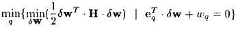 求解完成后对 w q w_q wq 进行剪枝即可。为了解上式,可以将其写为拉格朗日展式:
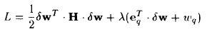 对其求解可以得到 optimal weight change 和 resulting change in error 分别为
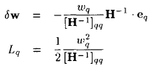
![[ICNN 1993] Optimal brain surgeon and general network pruning_第1张图片](http://img.e-com-net.com/image/info8/cd65380935c74a27aea141bb396339fa.png)
![[ICNN 1993] Optimal brain surgeon and general network pruning_第2张图片](http://img.e-com-net.com/image/info8/8ab68f3fc8f94786b04b109e6938f0e0.png)
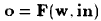 其中, i n \mathbf{in} in 为输入向量, w \mathbf{w} w 为权重, o \mathbf{o} o 为输出向量。训练集上的均方误差可以表示为
 由此可以计算出 w \mathbf{w} w 的一阶导
 注意上式中的 ∂ F ( w , i n [ k ] ) ∂ w ( t [ k ] − o [ k ] ) \frac{\partial F(\mathbf w,\mathbf {in}^{[k]})}{\partial \mathbf w}(\mathbf t^{[k]}-\mathbf o^{[k]}) ∂w∂F(w,in[k])(t[k]−o[k]) 为向量逐元素乘。进一步可以推出二阶导 / Hessian 为
![[ICNN 1993] Optimal brain surgeon and general network pruning_第3张图片](http://img.e-com-net.com/image/info8/ea8970382a074c36903bccd95e1e87df.png)
 令
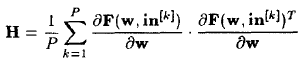
令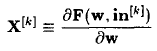 则得到了 Hessian matrix 的 outer-product approximation
 其中, P P P 为训练集样本数, X [ k ] \mathbf X^{[k]} X[k] 为第 k k k 个样本的 n n n-dimensional data vector of derivatives. 假如网络有多个输出,则 X \mathbf X X 为
 Hessian matrix 为
 其中, H 0 = α I H_0=\alpha I H0=αI, H P = H H_P=H HP=H
 将其代入 H H H 的迭代式可知,
 其中, H 0 − 1 = α − 1 I H^{-1}_0=\alpha^{-1}I H0−1=α−1I, H P − 1 = H − 1 H_P^{-1}=H^{-1} HP−1=H−1, α \alpha α ( 1 0 − 8 ≤ α ≤ 1 0 − 4 10^{-8}\leq\alpha\leq 10^{-4} 10−8≤α≤10−4) 为 a small constant needed to make H 0 − 1 H^{-1}_0 H0−1 meaningful.