【西瓜书笔记】8. EM算法(上)
EM算法的引入
引入EM算法的原因:
概率模型有时候既含有观测变量,又含有隐变量或者潜在变量。如果概率模型的变量都是观测变量,那么给定数据,可以直接用极大似然估计法,或者贝叶斯估计法估计模型参数。但是当模型含有隐变量时,就不能简单地使用这些估计方法。EM算法就是含有隐变量的概率模型参数的极大似然估计法。
EM算法的例子
《统计学习方法》例9.1(三硬币模型):
假设有3枚硬币,分别记作A,B,C。这些硬币正面出现的概率分别是 π \pi π , p p p 和 q q q 。进行如下掷硬币试验: 先掷硬币A,根据其结果选出硬币B或硬币C,正面选硬币B,反面选硬币C;然后掷选出的硬币,掷硬币的结果,出现正面记作1,出现反面记作0;独立地重复n次实验(这里,n=10),观测结果如下
1 , 1 , 0 , 1 , 0 , 0 , 1 , 0 , 1 , 1 1,1,0,1,0,0,1,0,1,1 1,1,0,1,0,0,1,0,1,1
假设只能观测到掷硬币的结果,不能观测掷硬币的过程。问如何估计三硬币正面出现的概率,即三硬币模型的参数。
对于每一次实验可以进行如下建模:
P ( y ∣ θ ) = ∑ z P ( y , z ∣ θ ) = ∑ z P ( z ∣ θ ) P ( y ∣ z , θ ) P(y \mid \theta)=\sum_{z} P(y, z \mid \theta)=\sum_{z} P(z \mid \theta) P(y \mid z, \theta) P(y∣θ)=z∑P(y,z∣θ)=z∑P(z∣θ)P(y∣z,θ)
随机变量y是观测变量,表示一次试验观测的结果是1或0;随机变量z是隐变量,表示未观测到的掷硬币A的结果。这里其实利用了 P ( A ) = ∑ B P ( A , B ) P(A)=\sum_{B}P(A, B) P(A)=∑BP(A,B),以及 P ( A , B ) = P ( A ) ⋅ P ( A ∣ B ) P(A, B)=P(A)\cdot P(A|B) P(A,B)=P(A)⋅P(A∣B)。然后我们有
P ( y ∣ θ ) = ∑ z P ( y , z ∣ θ ) = ∑ z P ( z ∣ θ ) P ( y ∣ z , θ ) = P ( z = 1 ∣ θ ) P ( y ∣ z = 1 , θ ) + P ( z = 0 ∣ θ ) P ( y ∣ z = 0 , θ ) = { π p + ( 1 − π ) q , if y = 1 π ( 1 − p ) + ( 1 − π ) ( 1 − q ) , if y = 0 = π p y ( 1 − p ) 1 − y + ( 1 − π ) q y ( 1 − q ) 1 − y \begin{aligned} P(y \mid \theta) &=\sum_{z} P(y, z \mid \theta)=\sum_{z} P(z \mid \theta) P(y \mid z, \theta) \\ &=P(z=1 \mid \theta) P(y \mid z=1, \theta)+P(z=0 \mid \theta) P(y \mid z=0, \theta) \\ &= \begin{cases}\pi p+(1-\pi) q, & \text { if } y=1 \\ \pi(1-p)+(1-\pi)(1-q), & \text { if } y=0\end{cases} \\ &=\pi p^{y}(1-p)^{1-y}+(1-\pi) q^{y}(1-q)^{1-y} \end{aligned} P(y∣θ)=z∑P(y,z∣θ)=z∑P(z∣θ)P(y∣z,θ)=P(z=1∣θ)P(y∣z=1,θ)+P(z=0∣θ)P(y∣z=0,θ)={πp+(1−π)q,π(1−p)+(1−π)(1−q), if y=1 if y=0=πpy(1−p)1−y+(1−π)qy(1−q)1−y
这里 θ = ( π , p , q ) \theta=(\pi, p, q) θ=(π,p,q)是模型参数。将观测数据表示为 Y = ( Y 1 , Y 2 , … , Y n ) T Y=\left(Y_{1}, Y_{2}, \ldots, Y_{n}\right)^{T} Y=(Y1,Y2,…,Yn)T,未观测数据表示为 Z = ( Z 1 , Z 2 , … , Z n ) T Z=\left(Z_{1}, Z_{2}, \ldots, Z_{n}\right)^{T} Z=(Z1,Z2,…,Zn)T,则观测数据的似然函数为每次实验累乘的结果:
P ( Y ∣ θ ) = ∑ Z P ( Z ∣ θ ) P ( Y ∣ Z , θ ) = ∏ j = 1 n P ( y j ∣ θ ) = ∏ j = 1 n [ π p y j ( 1 − p ) 1 − y j + ( 1 − π ) q y j ( 1 − q ) 1 − y j ] P(Y \mid \theta)=\sum_{Z} P(Z \mid \theta) P(Y \mid Z, \theta)=\prod_{j=1}^{n} P\left(y_{j} \mid \theta\right)\\ =\prod_{j=1}^{n}\left[\pi p^{y_{j}}(1-p)^{1-y_{j}}+(1-\pi) q^{y_{j}}(1-q)^{1-y_{j}}\right] P(Y∣θ)=Z∑P(Z∣θ)P(Y∣Z,θ)=j=1∏nP(yj∣θ)=j=1∏n[πpyj(1−p)1−yj+(1−π)qyj(1−q)1−yj]
考虑求模型参数 θ = ( π , p , q ) \theta=(\pi, p, q) θ=(π,p,q)的极大似然估计,也就是使用对数似然函数来进行参数估计可得:
θ ^ = arg max θ ln P ( Y ∣ θ ) = arg max θ ln ∏ j = 1 n [ π p y j ( 1 − p ) 1 − y j + ( 1 − π ) q y j ( 1 − q ) 1 − y j ] = arg max θ ∑ j = 1 n ln [ π p y j ( 1 − p ) 1 − y j + ( 1 − π ) q y j ( 1 − q ) 1 − y j ] \begin{aligned} \hat{\theta} &=\arg \max _{\theta} \ln P(Y \mid \theta) \\ &=\arg \max _{\theta} \ln \prod_{j=1}^{n}\left[\pi p^{y_{j}}(1-p)^{1-y_{j}}+(1-\pi) q^{y_{j}}(1-q)^{1-y_{j}}\right] \\ &=\arg \max _{\theta} \sum_{j=1}^{n} \ln \left[\pi p^{y_{j}}(1-p)^{1-y_{j}}+(1-\pi) q^{y_{j}}(1-q)^{1-y_{j}}\right] \end{aligned} θ^=argθmaxlnP(Y∣θ)=argθmaxlnj=1∏n[πpyj(1−p)1−yj+(1−π)qyj(1−q)1−yj]=argθmaxj=1∑nln[πpyj(1−p)1−yj+(1−π)qyj(1−q)1−yj]
上式没有解析解,也就是没办法直接解出 π , p , q \pi, p, q π,p,q恰好等于某个常数a, b, c。因此我们只能用迭代的方法进行求解。
EM算法的导出
Jesen(琴生)不等式:
若 f f f是凸函数,则:
f ( t x 1 + ( 1 − t ) x 2 ) ≤ t f ( x 1 ) + ( 1 − t ) f ( x 2 ) f\left(t x_{1}+(1-t) x_{2}\right) \leq t f\left(x_{1}\right)+(1-t) f\left(x_{2}\right) f(tx1+(1−t)x2)≤tf(x1)+(1−t)f(x2)
其中, t ∈ [ 0 , 1 ] t \in[0,1] t∈[0,1]。同理,如果 f f f是凹函数,则只需将上式中的 ≤ \leq ≤换成 ≥ \geq ≥即可。
将上式中的 t t t推广到 n n n个变量,同样成立:
f ( t 1 x 1 + t 2 x 2 + … + t n x n ) ≤ t 1 f ( x 1 ) + t 2 f ( x 2 ) + … + t n f ( x n ) f\left(t_{1} x_{1}+t_{2} x_{2}+\ldots+t_{n} x_{n}\right) \leq t_{1} f\left(x_{1}\right)+t_{2} f\left(x_{2}\right)+\ldots+t_{n} f\left(x_{n}\right) f(t1x1+t2x2+…+tnxn)≤t1f(x1)+t2f(x2)+…+tnf(xn)
其中, t 1 , t 2 , … , t n ∈ [ 0 , 1 ] , t 1 + t 2 + … + t n = 1 t_{1}, t_{2}, \ldots, t_{n} \in[0,1], t_{1}+t_{2}+\ldots+t_{n}=1 t1,t2,…,tn∈[0,1],t1+t2+…+tn=1. 在概率论中常以以下形式出现
φ ( E [ X ] ) ≤ E [ φ ( X ) ] \varphi(E[X]) \leq E[\varphi(X)] φ(E[X])≤E[φ(X)]
其中, X X X是随机变量, φ \varphi φ是凸函数, E [ X ] E[X] E[X]表示 X X X的期望。
我们面对一个含有隐变量的概率模型,目标是极大化观测数据Y关于参数θ的对数似然 函数,即极大化:
L ( θ ) = ln P ( Y ∣ θ ) = ln ∑ Z P ( Y , Z ∣ θ ) = ln ( ∑ Z P ( Y ∣ Z , θ ) P ( Z ∣ θ ) ) L(\theta)=\ln P(Y \mid \theta)=\ln \sum_{Z} P(Y, Z \mid \theta)=\ln \left(\sum_{Z} P(Y \mid Z, \theta) P(Z \mid \theta)\right) L(θ)=lnP(Y∣θ)=lnZ∑P(Y,Z∣θ)=ln(Z∑P(Y∣Z,θ)P(Z∣θ))
注意到这一极大化的主要困难是上式中有未观测数据Z并有包含和(Z为离散型时)或者积分(Z为连续型时)的对数。EM算法采用的是通过迭代逐步近似极大化 L ( θ ) L(\theta) L(θ)。假设在第i次迭代后 θ \theta θ的估计值是 θ ( i ) \theta^{(i)} θ(i),我们希望新的估计值 θ \theta θ能够使 L ( θ ) L(\theta) L(θ)增加,即 L ( θ ) > L ( θ ( i ) ) L(\theta)>L\left(\theta^{(i)}\right) L(θ)>L(θ(i))并逐步达到极大值。为此,我们考虑两者的差:
L ( θ ) − L ( θ ( i ) ) = ln ( ∑ Z P ( Y ∣ Z , θ ) P ( Z ∣ θ ) ) − ln P ( Y ∣ θ ( i ) ) = ln ( ∑ Z P ( Z ∣ Y , θ ( i ) ) P ( Y ∣ Z , θ ) P ( Z ∣ θ ) P ( Z ∣ Y , θ ( i ) ) ) − ln P ( Y ∣ θ ( i ) ) \begin{aligned} L(\theta)-L\left(\theta^{(i)}\right) &=\ln \left(\sum_{Z} P(Y \mid Z, \theta) P(Z \mid \theta)\right)-\ln P\left(Y \mid \theta^{(i)}\right) \\ &=\ln \left(\sum_{Z} P\left(Z \mid Y, \theta^{(i)}\right) \frac{P(Y \mid Z, \theta) P(Z \mid \theta)}{P\left(Z \mid Y, \theta^{(i)}\right)}\right)-\ln P\left(Y \mid \theta^{(i)}\right) \end{aligned} L(θ)−L(θ(i))=ln(Z∑P(Y∣Z,θ)P(Z∣θ))−lnP(Y∣θ(i))=ln(Z∑P(Z∣Y,θ(i))P(Z∣Y,θ(i))P(Y∣Z,θ)P(Z∣θ))−lnP(Y∣θ(i))
套用琴生不等式可有
ln ( ∑ Z P ( Z ∣ Y , θ ( i ) ) P ( Y ∣ Z , θ ) P ( Z ∣ θ ) P ( Z ∣ Y , θ ( i ) ) ) − ln P ( Y ∣ θ ( i ) ) ≥ ∑ Z P ( Z ∣ Y , θ ( i ) ) ln P ( Y ∣ Z , θ ) P ( Z ∣ θ ) P ( Z ∣ Y , θ ( i ) ) − ln P ( Y ∣ θ ( i ) ) = ∑ Z P ( Z ∣ Y , θ ( i ) ) ln P ( Y ∣ Z , θ ) P ( Z ∣ θ ) P ( Z ∣ Y , θ ( i ) ) − 1 ⋅ ln P ( Y ∣ θ ( i ) ) \begin{aligned} &\ln \left(\sum_{Z} P\left(Z \mid Y, \theta^{(i)}\right) \frac{P(Y \mid Z, \theta) P(Z \mid \theta)}{P\left(Z \mid Y, \theta^{(i)}\right)}\right)-\ln P\left(Y \mid \theta^{(i)}\right)\\ &\geq \sum_{Z} P\left(Z \mid Y, \theta^{(i)}\right) \ln \frac{P(Y \mid Z, \theta) P(Z \mid \theta)}{P\left(Z \mid Y, \theta^{(i)}\right)}-\ln P\left(Y \mid \theta^{(i)}\right) \\ &=\sum_{Z} P\left(Z \mid Y, \theta^{(i)}\right) \ln \frac{P(Y \mid Z, \theta) P(Z \mid \theta)}{P\left(Z \mid Y, \theta^{(i)}\right)}-1 \cdot \ln P\left(Y \mid \theta^{(i)}\right) \end{aligned} ln(Z∑P(Z∣Y,θ(i))P(Z∣Y,θ(i))P(Y∣Z,θ)P(Z∣θ))−lnP(Y∣θ(i))≥Z∑P(Z∣Y,θ(i))lnP(Z∣Y,θ(i))P(Y∣Z,θ)P(Z∣θ)−lnP(Y∣θ(i))=Z∑P(Z∣Y,θ(i))lnP(Z∣Y,θ(i))P(Y∣Z,θ)P(Z∣θ)−1⋅lnP(Y∣θ(i))
这里 P ( Z ∣ Y , θ ( i ) ) P\left(Z \mid Y, \theta^{(i)}\right) P(Z∣Y,θ(i))相当于式(7)中的 t i t_i ti,对数函数相当于 f f f。这不过这里是凹函数,所以不等式方向相反。又因为 1 = ∑ Z P ( Z ∣ Y , θ ( i ) ) 1=\sum_{Z} P\left(Z \mid Y, \theta^{(i)}\right) 1=∑ZP(Z∣Y,θ(i))于是
L ( θ ) − L ( θ ( i ) ) ≥ ∑ Z P ( Z ∣ Y , θ ( i ) ) ln P ( Y ∣ Z , θ ) P ( Z ∣ θ ) P ( Z ∣ Y , θ ( i ) ) − ∑ Z P ( Z ∣ Y , θ ( i ) ) ⋅ ln P ( Y ∣ θ ( i ) ) = ∑ Z P ( Z ∣ Y , θ ( i ) ) ( ln P ( Y ∣ Z , θ ) P ( Z ∣ θ ) P ( Z ∣ Y , θ ( i ) ) − ln P ( Y ∣ θ ( i ) ) ) = ∑ Z P ( Z ∣ Y , θ ( i ) ) ln P ( Y ∣ Z , θ ) P ( Z ∣ θ ) P ( Z ∣ Y , θ ( i ) ) P ( Y ∣ θ ( i ) ) \begin{aligned} L(\theta)-L\left(\theta^{(i)}\right) & \geq \sum_{Z} P\left(Z \mid Y, \theta^{(i)}\right) \ln \frac{P(Y \mid Z, \theta) P(Z \mid \theta)}{P\left(Z \mid Y, \theta^{(i)}\right)}-\sum_{Z} P\left(Z \mid Y, \theta^{(i)}\right) \cdot \ln P\left(Y \mid \theta^{(i)}\right) \\ &=\sum_{Z} P\left(Z \mid Y, \theta^{(i)}\right)\left(\ln \frac{P(Y \mid Z, \theta) P(Z \mid \theta)}{P\left(Z \mid Y, \theta^{(i)}\right)}-\ln P\left(Y \mid \theta^{(i)}\right)\right) \\ &=\sum_{Z} P\left(Z \mid Y, \theta^{(i)}\right) \ln \frac{P(Y \mid Z, \theta) P(Z \mid \theta)}{P\left(Z \mid Y, \theta^{(i)}\right) P\left(Y \mid \theta^{(i)}\right)} \end{aligned} L(θ)−L(θ(i))≥Z∑P(Z∣Y,θ(i))lnP(Z∣Y,θ(i))P(Y∣Z,θ)P(Z∣θ)−Z∑P(Z∣Y,θ(i))⋅lnP(Y∣θ(i))=Z∑P(Z∣Y,θ(i))(lnP(Z∣Y,θ(i))P(Y∣Z,θ)P(Z∣θ)−lnP(Y∣θ(i)))=Z∑P(Z∣Y,θ(i))lnP(Z∣Y,θ(i))P(Y∣θ(i))P(Y∣Z,θ)P(Z∣θ)
所以
L ( θ ) ≥ L ( θ ( i ) ) + ∑ Z P ( Z ∣ Y , θ ( i ) ) ln P ( Y ∣ Z , θ ) P ( Z ∣ θ ) P ( Z ∣ Y , θ ( i ) ) P ( Y ∣ θ ( i ) ) L(\theta) \geq L\left(\theta^{(i)}\right)+\sum_{Z} P\left(Z \mid Y, \theta^{(i)}\right) \ln \frac{P(Y \mid Z, \theta) P(Z \mid \theta)}{P\left(Z \mid Y, \theta^{(i)}\right) P\left(Y \mid \theta^{(i)}\right)} L(θ)≥L(θ(i))+Z∑P(Z∣Y,θ(i))lnP(Z∣Y,θ(i))P(Y∣θ(i))P(Y∣Z,θ)P(Z∣θ)
令
B ( θ , θ ( i ) ) = L ( θ ( i ) ) + ∑ Z P ( Z ∣ Y , θ ( i ) ) ln P ( Y ∣ Z , θ ) P ( Z ∣ θ ) P ( Z ∣ Y , θ ( i ) ) P ( Y ∣ θ ( i ) ) B\left(\theta, \theta^{(i)}\right)=L\left(\theta^{(i)}\right)+\sum_{Z} P\left(Z \mid Y, \theta^{(i)}\right) \ln \frac{P(Y \mid Z, \theta) P(Z \mid \theta)}{P\left(Z \mid Y, \theta^{(i)}\right) P\left(Y \mid \theta^{(i)}\right)} B(θ,θ(i))=L(θ(i))+Z∑P(Z∣Y,θ(i))lnP(Z∣Y,θ(i))P(Y∣θ(i))P(Y∣Z,θ)P(Z∣θ)
则有
L ( θ ) ≥ B ( θ , θ ( i ) ) L(\theta) \geq B\left(\theta, \theta^{(i)}\right) L(θ)≥B(θ,θ(i))
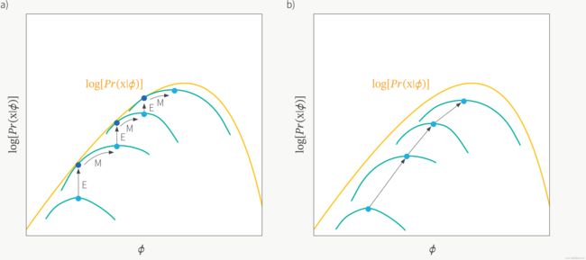
在第一次迭代的时候, θ i \theta_i θi都是随机初始化的,通常初始化为 π = p = q = 0.5 \pi=p=q=0.5 π=p=q=0.5。现在我们不去极大化 L ( θ ) L(\theta) L(θ),因为前面说过这很困难。我们转而去极大化它的下界 B ( θ , θ ( i ) ) B\left(\theta, \theta^{(i)}\right) B(θ,θ(i)),得到一个新的 θ \theta θ,然后把这个新的 θ \theta θ代入到 L ( θ ) L(\theta) L(θ),看是不是能使得 L ( θ ) L(\theta) L(θ)变大。也就说 B ( θ , θ ( i ) ) B\left(\theta, \theta^{(i)}\right) B(θ,θ(i))是 L ( θ ) L(\theta) L(θ)的一个下界,此时若设 θ ( i + 1 ) \theta^{(i+1)} θ(i+1)使得 B ( θ , θ ( i ) ) B\left(\theta, \theta^{(i)}\right) B(θ,θ(i))达到极大(不是最大),也即
B ( θ ( i + 1 ) , θ ( i ) ) ≥ B ( θ ( i ) , θ ( i ) ) B\left(\theta^{(i+1)}, \theta^{(i)}\right) \geq B\left(\theta^{(i)}, \theta^{(i)}\right) B(θ(i+1),θ(i))≥B(θ(i),θ(i))
进一步可得
L ( θ ( i + 1 ) ) ≥ B ( θ ( i + 1 ) , θ ( i ) ) ≥ B ( θ ( i ) , θ ( i ) ) = L ( θ ( i ) ) ⇒ L ( θ ( i + 1 ) ) ≥ L ( θ ( i ) ) L\left(\theta^{(i+1)}\right) \geq B\left(\theta^{(i+1)}, \theta^{(i)}\right) \geq B\left(\theta^{(i)}, \theta^{(i)}\right)=L\left(\theta^{(i)}\right)\\ \Rightarrow L\left(\theta^{(i+1)}\right) \geq L\left(\theta^{(i)}\right) L(θ(i+1))≥B(θ(i+1),θ(i))≥B(θ(i),θ(i))=L(θ(i))⇒L(θ(i+1))≥L(θ(i))
这里注意:
B ( θ ( i ) , θ ( i ) ) = L ( θ ( i ) ) + ∑ Z P ( Z ∣ Y , θ ( i ) ) ln P ( Y ∣ Z , θ ( i ) ) P ( Z ∣ θ ( i ) ) P ( Z ∣ Y , θ ( i ) ) P ( Y ∣ θ ( i ) ) = L ( θ ( i ) ) + ∑ Z P ( Z ∣ Y , θ ( i ) ) ln P ( Y , Z ∣ θ ( i ) ) P ( Y , Z ∣ θ ( i ) ) = L ( θ ( i ) ) B\left(\theta^{(i)}, \theta^{(i)}\right)=L\left(\theta^{(i)}\right)+\sum_{Z} P\left(Z \mid Y, \theta^{(i)}\right) \ln \frac{P(Y \mid Z, \theta^{(i)}) P(Z \mid \theta^{(i)})}{P\left(Z \mid Y, \theta^{(i)}\right) P\left(Y \mid \theta^{(i)}\right)}\\ =L\left(\theta^{(i)}\right)+\sum_{Z} P\left(Z \mid Y, \theta^{(i)}\right) \ln \frac{P(Y, Z\mid\theta^{(i)})}{P(Y, Z\mid\theta^{(i)})}\\ =L(\theta^{(i)}) B(θ(i),θ(i))=L(θ(i))+Z∑P(Z∣Y,θ(i))lnP(Z∣Y,θ(i))P(Y∣θ(i))P(Y∣Z,θ(i))P(Z∣θ(i))=L(θ(i))+Z∑P(Z∣Y,θ(i))lnP(Y,Z∣θ(i))P(Y,Z∣θ(i))=L(θ(i))
所以,任何可以使 B ( θ , θ ( i ) ) B(\theta, \theta^{(i)}) B(θ,θ(i))增大的 θ \theta θ,也可使 L ( θ ) L(\theta) L(θ)增大,于是问题转化为了求解能使得 B ( θ , θ ( i ) ) B\left(\theta, \theta^{(i)}\right) B(θ,θ(i))达到极大的 θ ( i + 1 ) \theta^{(i+1)} θ(i+1),即
θ ( i + 1 ) = arg max θ B ( θ , θ ( i ) ) = arg max θ ( L ( θ ( i ) ) + ∑ Z P ( Z ∣ Y , θ ( i ) ) ln P ( Y ∣ Z , θ ) P ( Z ∣ θ ) P ( Z ∣ Y , θ ( i ) ) P ( Y ∣ θ ( i ) ) ) = arg max θ ( ∑ Z P ( Z ∣ Y , θ ( i ) ) ln ( P ( Y ∣ Z , θ ) P ( Z ∣ θ ) ) ) = arg max θ ( ∑ Z P ( Z ∣ Y , θ ( i ) ) ln P ( Y , Z ∣ θ ) ) = arg max θ Q ( θ , θ ( i ) ) \begin{aligned} \theta^{(i+1)} &=\underset{\theta}{\arg \max } B\left(\theta, \theta^{(i)}\right) \\ &=\underset{\theta}{\arg \max }\left(L\left(\theta^{(i)}\right)+\sum_{Z} P\left(Z \mid Y, \theta^{(i)}\right) \ln \frac{P(Y \mid Z, \theta) P(Z \mid \theta)}{P\left(Z \mid Y, \theta^{(i)}\right) P\left(Y \mid \theta^{(i)}\right)}\right) \\ &=\underset{\theta}{\arg \max }\left(\sum_{Z} P\left(Z \mid Y, \theta^{(i)}\right) \ln (P(Y \mid Z, \theta) P(Z \mid \theta))\right) \\ &=\underset{\theta}{\arg \max }\left(\sum_{Z} P\left(Z \mid Y, \theta^{(i)}\right) \ln P(Y, Z \mid \theta)\right) \\ &=\underset{\theta}{\arg \max } Q\left(\theta, \theta^{(i)}\right) \end{aligned} θ(i+1)=θargmaxB(θ,θ(i))=θargmax(L(θ(i))+Z∑P(Z∣Y,θ(i))lnP(Z∣Y,θ(i))P(Y∣θ(i))P(Y∣Z,θ)P(Z∣θ))=θargmax(Z∑P(Z∣Y,θ(i))ln(P(Y∣Z,θ)P(Z∣θ)))=θargmax(Z∑P(Z∣Y,θ(i))lnP(Y,Z∣θ))=θargmaxQ(θ,θ(i))
到此即完成了EM算法的一次迭代,求出的 θ ( i + 1 ) \theta^{(i+1)} θ(i+1)作为下一次迭代的初始 θ ( i ) \theta^{(i)} θ(i)。综上可以总结出EM算法的“E步”和“M步”分别为:
-
E步:计算完全数据的对数似然函数 ln P ( Y , Z ∣ θ ) \ln P(Y, Z \mid \theta) lnP(Y,Z∣θ)关于在给定观测数据 Y Y Y和当前参数 θ \theta θ下对未观测数据 Z Z Z的条件概率分布 P ( Z ∣ Y , θ ( i ) ) P\left(Z \mid Y, \theta^{(i)}\right) P(Z∣Y,θ(i))的期望,也就是Q函数
Q ( θ , θ ( i ) ) = E Z [ ln P ( Y , Z ∣ θ ) ∣ Y , θ ( i ) ] = ∑ Z P ( Z ∣ Y , θ ( i ) ) ln P ( Y , Z ∣ θ ) Q\left(\theta, \theta^{(i)}\right)=E_{Z}\left[\ln P(Y, Z \mid \theta) \mid Y, \theta^{(i)}\right]=\sum_{Z} P\left(Z \mid Y, \theta^{(i)}\right) \ln P(Y, Z \mid \theta) Q(θ,θ(i))=EZ[lnP(Y,Z∣θ)∣Y,θ(i)]=Z∑P(Z∣Y,θ(i))lnP(Y,Z∣θ) -
M步:求使得Q函数到达极大的 θ ( i + 1 ) \theta^{(i+1)} θ(i+1).
(souce:https://www.borealisai.com/en/blog/tutorial-5-variational-auto-encoders/)