python：pyGAM使用教程

作者：CSDN @ _养乐多_

本文记录了pyGAM库的使用方法和示例代码。包括GAM (构建自定义模型的基类)
LinearGAM、LogisticGAM、GammaGAM、PoissonGAM、InvGaussGAM、ExpectileGAM。

---

---

一、介绍

广义加性模型 (GAM) 是以下形式的平滑半参数模型：

$$g(E[y|X])=\beta 0+f1(X1)+f2(X2,X3)+\dots +fM(XN)$$

其中X.T = [X_1, X_2, ..., X_N]是自变量，y是因变量，g()是将我们的预测变量与因变量的预期值相关联的链接函数。

特征函数 f_i() 使用惩罚 B 样条构建，这使我们能够自动建模非线性关系，而无需手动尝试对每个变量进行许多不同的转换。

广义可加模型（GAMs）通过允许特征的非线性函数来扩展广义线性模型，同时保持可加性。由于该模型是可加的，因此可以很容易地在保持其他预测变量不变的情况下，单独检查每个 X_i 对 Y 的影响。

结果是一个非常灵活的模型，可以轻松地结合先验知识并控制过拟合。

$$y\sim ExponentialFamily(\mu |X)$$

这里

$$g(\mu |X)=\beta 0+f1(X1)+f2(X2,X3)+\dots +fM(XN)$$

因此，我们可以看到广义可加模型（GAM）包括三个组成部分：

• distribution 来自指数族
• link function $g(\cdot )$
• functional form 具有附加结构$\beta 0+f1(X1)+f2(X2,X3)+\dots +fM(XN)$

分配

指定方式：GAM(distribution='...')

目前您可以从以下选项中进行选择：

• 'normal'
• 'binomial'
• 'poisson'
• 'gamma'
• 'inv_gauss'

链接功能

我们指定使用：GAM(link='...')

链接函数将分布均值用于线性预测。到目前为止，可以使用以下内容：

• 'identity'
• 'logit'
• 'inverse'
• 'log'
• 'inverse-squared'

功能形式

指定GAM(terms=...)或更简单GAM(...)

在 pyGAM 中，我们使用术语指定函数形式：

• l()线性项：对于像Xi
• s()样条项
• f()因子项
• te()张量积
• intercept

有了这些，我们可以快速而紧凑地构建模型，例如：

from pygam import GAM, s, te

GAM(s(0, n_splines=200) + te(3,1) + s(2), distribution='poisson', link='log')

GAM(callbacks=[‘deviance’, ‘diffs’], distribution=‘poisson’,
fit_intercept=True, link=‘log’, max_iter=100,
terms=s(0) + te(3, 1) + s( 2), tol=0.0001, verbose=False)
它指定我们想要一个：

• 特征 0 上的样条函数，具有 200 个基函数
• 特征 1 和 3 上的张量样条相互作用
• 特征 2 上的样条函数

笔记：

GAM(..., intercept=True)所以模型默认包含截距。

二、在实践中

在pyGAM中，您可以通过指定这三个元素来构建自定义模型，或者您可以从常见的模型中进行选择：

• LinearGAM身份链接和正态分布
• LogisticGAMLogit 链接和二项分布
• PoissonGAM日志链接和泊松分布
• GammaGAM日志链接和伽玛分布
• InvGauss日志链接和 inv_gauss 分布

通用模型的好处是除了减少样板代码外，它们还有一些额外的特性。

项（Terms）和交互作用（Interactions）

项（Terms）和交互作用（Interactions）是GAM中的重要概念。

在GAM中，一个项表示一个预测变量与响应变量之间的关系。一个项可以是一个线性项，例如β0或β1*X1，也可以是一个非线性项，例如f1(X1)。通过组合多个项，可以建立一个包含多个预测变量的模型。

交互作用是指两个或多个预测变量之间的相互作用效应。在GAM中，可以通过引入交互项来捕捉这种效应。例如，一个交互项可以表示为f2(X2, X3)，它表示预测变量X2和X3之间的相互作用对响应变量的影响。

通过选择和组合不同的项和交互作用，可以建立一个灵活且富有解释力的GAM模型，以更好地理解预测变量与响应变量之间的关系。

pyGAM还可以通过使用te()函数来拟合通过张量积表示的交互作用。

from pygam import PoissonGAM, s, te
from pygam.datasets import chicago

X, y = chicago(return_X_y=True)

gam = PoissonGAM(s(0, n_splines=200) + te(3, 1) + s(2)).fit(X, y)

以及绘制3D表面：

import matplotlib.pyplot as plt
from mpl_toolkits import mplot3d

plt.ion()
plt.rcParams['figure.figsize'] = (12, 8)

XX = gam.generate_X_grid(term=1, meshgrid=True)
Z = gam.partial_dependence(term=1, X=XX, meshgrid=True)

ax = plt.axes(projection='3d')
ax.plot_surface(XX[0], XX[1], Z, cmap='viridis')

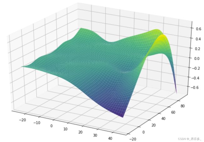
对于简单的交互作用，有时将一个by变量添加到一个项中是有用的。

from pygam import LinearGAM, s
from pygam.datasets import toy_interaction

X, y = toy_interaction(return_X_y=True)

gam = LinearGAM(s(0, by=1)).fit(X, y)
gam.summary()

LinearGAM
=============================================== ==========================================================
Distribution:                        NormalDist Effective DoF:                                     20.8449
Link Function:                     IdentityLink Log Likelihood:                              -2317525.6219
Number of Samples:                        50000 AIC:                                          4635094.9336
                                                AICc:                                         4635094.9536
                                                GCV:                                                  0.01
                                                Scale:                                                0.01
                                                Pseudo R-Squared:                                   0.9976
==========================================================================================================
Feature Function                  Lambda               Rank         EDoF         P > x        Sig. Code
================================= ==================== ============ ============ ============ ============
s(0)                              [0.6]                20           19.8         1.11e-16     ***
intercept                                              1            1.0          1.79e-01
==========================================================================================================
Significance codes:  0 '***' 0.001 '**' 0.01 '*' 0.05 '.' 0.1 ' ' 1

WARNING: Fitting splines and a linear function to a feature introduces a model identifiability problem
         which can cause p-values to appear significant when they are not.

WARNING: p-values calculated in this manner behave correctly for un-penalized models or models with
         known smoothing parameters, but when smoothing parameters have been estimated, the p-values
         are typically lower than they should be, meaning that the tests reject the null too readily.

回归

对于回归问题，我们可以使用线性GAM，它对以下内容进行建模：

$$E[y|X]=\beta 0+f1(X1)+f2(X2,X3)+\cdots +fM(XN)$$

from pygam import LinearGAM, s, f
from pygam.datasets import wage

X, y = wage(return_X_y=True)

## model
gam = LinearGAM(s(0) + s(1) + f(2))
gam.gridsearch(X, y)


## plotting
plt.figure();
fig, axs = plt.subplots(1,3);

titles = ['year', 'age', 'education']
for i, ax in enumerate(axs):
    XX = gam.generate_X_grid(term=i)
    ax.plot(XX[:, i], gam.partial_dependence(term=i, X=XX))
    ax.plot(XX[:, i], gam.partial_dependence(term=i, X=XX, width=.95)[1], c='r', ls='--')
    if i == 0:
        ax.set_ylim(-30,30)
    ax.set_title(titles[i]);

尽管我们的模型允许使用系数，但平滑惩罚将我们限制在仅有19个有效自由度：

gam.summary()

LinearGAM
=============================================== ==========================================================
Distribution:                        NormalDist Effective DoF:                                     19.2602
Link Function:                     IdentityLink Log Likelihood:                                -24116.7451
Number of Samples:                         3000 AIC:                                            48274.0107
                                                AICc:                                           48274.2999
                                                GCV:                                             1250.3656
                                                Scale:                                           1235.9245
                                                Pseudo R-Squared:                                   0.2945
==========================================================================================================
Feature Function                  Lambda               Rank         EDoF         P > x        Sig. Code
================================= ==================== ============ ============ ============ ============
s(0)                              [15.8489]            20           6.9          5.52e-03     **
s(1)                              [15.8489]            20           8.5          1.11e-16     ***
f(2)                              [15.8489]            5            3.8          1.11e-16     ***
intercept                         0                    1            0.0          1.11e-16     ***
==========================================================================================================
Significance codes:  0 '***' 0.001 '**' 0.01 '*' 0.05 '.' 0.1 ' ' 1

WARNING: Fitting splines and a linear function to a feature introduces a model identifiability problem
         which can cause p-values to appear significant when they are not.

WARNING: p-values calculated in this manner behave correctly for un-penalized models or models with
         known smoothing parameters, but when smoothing parameters have been estimated, the p-values
         are typically lower than they should be, meaning that the tests reject the null too readily.

使用LinearGAMs，我们还可以检查预测区间:

from pygam import LinearGAM
from pygam.datasets import mcycle

X, y = mcycle(return_X_y=True)

gam = LinearGAM(n_splines=25).gridsearch(X, y)
XX = gam.generate_X_grid(term=0, n=500)

plt.plot(XX, gam.predict(XX), 'r--')
plt.plot(XX, gam.prediction_intervals(XX, width=.95), color='b', ls='--')

plt.scatter(X, y, facecolor='gray', edgecolors='none')
plt.title('95% prediction interval');

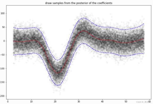
然后从后面进行模拟:

# continuing last example with the mcycle dataset
for response in gam.sample(X, y, quantity='y', n_draws=50, sample_at_X=XX):
    plt.scatter(XX, response, alpha=.03, color='k')
plt.plot(XX, gam.predict(XX), 'r--')
plt.plot(XX, gam.prediction_intervals(XX, width=.95), color='b', ls='--')
plt.title('draw samples from the posterior of the coefficients')

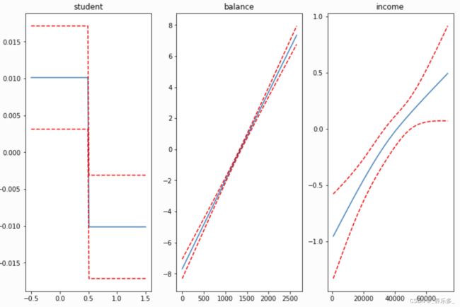
分类

对于二元分类问题，我们可以使用logistic GAM模型:

$$log(P(y=1|X)P(y=0|X))=\beta 0+f1(X1)+f2(X2,X3)+\cdots +fM(XN)$$

from pygam import LogisticGAM, s, f
from pygam.datasets import default

X, y = default(return_X_y=True)

gam = LogisticGAM(f(0) + s(1) + s(2)).gridsearch(X, y)

fig, axs = plt.subplots(1, 3)
titles = ['student', 'balance', 'income']

for i, ax in enumerate(axs):
    XX = gam.generate_X_grid(term=i)
    pdep, confi = gam.partial_dependence(term=i, width=.95)

    ax.plot(XX[:, i], pdep)
    ax.plot(XX[:, i], confi, c='r', ls='--')
    ax.set_title(titles[i]);

gam.accuracy(X, y)

由于二项分布的规模是已知的，我们的网格搜索最小化了无偏风险估计器(UBRE)的目标:

gam.summary()

LogisticGAM
=============================================== ==========================================================
Distribution:                      BinomialDist Effective DoF:                                      3.8047
Link Function:                        LogitLink Log Likelihood:                                   -788.877
Number of Samples:                        10000 AIC:                                             1585.3634
                                                AICc:                                             1585.369
                                                UBRE:                                               2.1588
                                                Scale:                                                 1.0
                                                Pseudo R-Squared:                                   0.4598
==========================================================================================================
Feature Function                  Lambda               Rank         EDoF         P > x        Sig. Code
================================= ==================== ============ ============ ============ ============
f(0)                              [1000.]              2            1.7          4.61e-03     **
s(1)                              [1000.]              20           1.2          0.00e+00     ***
s(2)                              [1000.]              20           0.8          3.29e-02     *
intercept                         0                    1            0.0          0.00e+00     ***
==========================================================================================================
Significance codes:  0 '***' 0.001 '**' 0.01 '*' 0.05 '.' 0.1 ' ' 1

WARNING: Fitting splines and a linear function to a feature introduces a model identifiability problem
         which can cause p-values to appear significant when they are not.

WARNING: p-values calculated in this manner behave correctly for un-penalized models or models with
         known smoothing parameters, but when smoothing parameters have been estimated, the p-values
         are typically lower than they should be, meaning that the tests reject the null too readily.

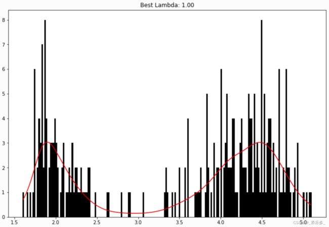
泊松和直方图平滑

我们可以直观地执行直方图平滑，通过PoissonGAM将每个bin中的计数建模为分布泊松。

from pygam import PoissonGAM
from pygam.datasets import faithful

X, y = faithful(return_X_y=True)

gam = PoissonGAM().gridsearch(X, y)

plt.hist(faithful(return_X_y=False)['eruptions'], bins=200, color='k');
plt.plot(X, gam.predict(X), color='r')
plt.title('Best Lambda: {0:.2f}'.format(gam.lam[0][0]));

预测

具有正态分布的GAM模型存在假定方差恒定的局限性。有时这并不是一个适当的假设，因为我们希望误差分布的方差可以变化。

在这种情况下，我们可以转而建模分布的期望分位数。

期望分位数直观上类似于分位数，但是模型化的是尾部期望而不是尾部质量。尽管期望分位数的解释性较差，但拟合速度更快，并且还可以用于非参数地建模分布。

from pygam import ExpectileGAM
from pygam.datasets import mcycle

X, y = mcycle(return_X_y=True)

# lets fit the mean model first by CV
gam50 = ExpectileGAM(expectile=0.5).gridsearch(X, y)

# and copy the smoothing to the other models
lam = gam50.lam

# now fit a few more models
gam95 = ExpectileGAM(expectile=0.95, lam=lam).fit(X, y)
gam75 = ExpectileGAM(expectile=0.75, lam=lam).fit(X, y)
gam25 = ExpectileGAM(expectile=0.25, lam=lam).fit(X, y)
gam05 = ExpectileGAM(expectile=0.05, lam=lam).fit(X, y)

XX = gam50.generate_X_grid(term=0, n=500)

plt.scatter(X, y, c='k', alpha=0.2)
plt.plot(XX, gam95.predict(XX), label='0.95')
plt.plot(XX, gam75.predict(XX), label='0.75')
plt.plot(XX, gam50.predict(XX), label='0.50')
plt.plot(XX, gam25.predict(XX), label='0.25')
plt.plot(XX, gam05.predict(XX), label='0.05')
plt.legend()

我们通过交叉验证来拟合均值模型，以找到最佳的平滑参数lam，然后将其应用到其他模型中。

这种做法可以减少期望分位数之间的交叉。

自定义模型

通过使用基本GAM类并指定分布和链接函数来构建自定义模型也很容易：

from pygam import GAM
from pygam.datasets import trees

X, y = trees(return_X_y=True)

gam = GAM(distribution='gamma', link='log')
gam.gridsearch(X, y)

plt.scatter(y, gam.predict(X))
plt.xlabel('true volume')
plt.ylabel('predicted volume')

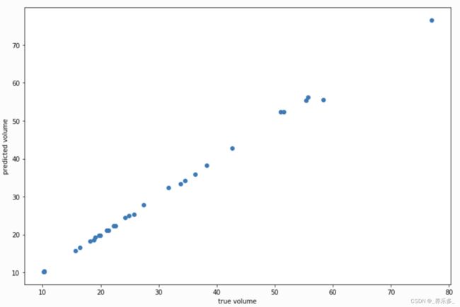
我们可以通过查看 Pseudo R-Squared 来检查拟合质量：

gam.summary()

GAM
=============================================== ==========================================================
Distribution:                         GammaDist Effective DoF:                                     25.3616
Link Function:                          LogLink Log Likelihood:                                   -26.1673
Number of Samples:                           31 AIC:                                              105.0579
                                                AICc:                                             501.5549
                                                GCV:                                                0.0088
                                                Scale:                                               0.001
                                                Pseudo R-Squared:                                   0.9993
==========================================================================================================
Feature Function                  Lambda               Rank         EDoF         P > x        Sig. Code
================================= ==================== ============ ============ ============ ============
s(0)                              [0.001]              20                        2.04e-08     ***
s(1)                              [0.001]              20                        7.36e-06     ***
intercept                         0                    1                         4.39e-13     ***
==========================================================================================================
Significance codes:  0 '***' 0.001 '**' 0.01 '*' 0.05 '.' 0.1 ' ' 1

WARNING: Fitting splines and a linear function to a feature introduces a model identifiability problem
         which can cause p-values to appear significant when they are not.

WARNING: p-values calculated in this manner behave correctly for un-penalized models or models with
         known smoothing parameters, but when smoothing parameters have been estimated, the p-values
         are typically lower than they should be, meaning that the tests reject the null too readily.

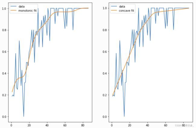
处罚/约束

使用 GAM，我们可以编码先验知识并通过使用惩罚和约束来控制过度拟合。

可用惩罚- 二阶导数平滑（数值特征默认） - L2 平滑（分类特征默认）

可用约束- 单调递增/递减平滑 - 凸/凹平滑 - 周期性平滑 [很快…]

我们可以通过使用单调和凹约束将我们的直觉注入我们的模型：

from pygam import LinearGAM, s
from pygam.datasets import hepatitis

X, y = hepatitis(return_X_y=True)

gam1 = LinearGAM(s(0, constraints='monotonic_inc')).fit(X, y)
gam2 = LinearGAM(s(0, constraints='concave')).fit(X, y)

fig, ax = plt.subplots(1, 2)
ax[0].plot(X, y, label='data')
ax[0].plot(X, gam1.predict(X), label='monotonic fit')
ax[0].legend()

ax[1].plot(X, y, label='data')
ax[1].plot(X, gam2.predict(X), label='concave fit')
ax[1].legend()

应用程序接口

pyGAM 直观、模块化，并遵循熟悉的 API：

from pygam import LogisticGAM, s, f
from pygam.datasets import toy_classification

X, y = toy_classification(return_X_y=True, n=5000)

gam = LogisticGAM(s(0) + s(1) + s(2) + s(3) + s(4) + f(5))
gam.fit(X, y)

由于GAM是可加模型，因此可以非常容易地可视化每个单独的特征函数f_i(X_i)。这些特征函数描述了每个X_i对y的影响，同时将所有其他预测变量边际化。

plt.figure()
for i, term in enumerate(gam.terms):
    if term.isintercept:
        continue
    plt.plot(gam.partial_dependence(term=i))

当前功能

模型

pyGAM 附带了许多即插即用的模型：

• GAM (构建自定义模型的基类)
• LinearGAM
• LogisticGAM
• GammaGAM
• PoissonGAM
• InvGaussGAM
• ExpectileGAM

terms

• l() linear terms
• s() spline terms
• f() factor terms
• te() tensor products
• intercept

分布

• Normal
• Binomial
• Gamma
• Poisson
• Inverse Gaussian

链接函数将分布的均值映射到线性预测。以下是上述分布的规范链接函数：

• 正态分布（Normal Distribution）：恒等链接函数（Identity Link Function）
• 二项分布（Binomial Distribution）：对数链接函数（Logit Link Function）
• 泊松分布（Poisson Distribution）：对数链接函数（Log Link Function）
• 伽马分布（Gamma Distribution）：倒数链接函数（Inverse Link Function）
• 逆高斯分布（Inverse Gaussian Distribution）：平方根链接函数（Inverse Square Root Link Function）
• 负二项分布（Negative Binomial Distribution）：对数链接函数（Log Link Function）

链接函数的选择取决于所使用的分布类型。每个分布都有一个与之关联的规范链接函数，它在将分布的均值映射到线性预测时起到关键作用。通过使用适当的链接函数，我们可以确保模型具有良好的数学性质，并与所选择的分布类型相匹配。

链接功能

• Identity
• Logit
• Inverse
• Log
• Inverse-squared

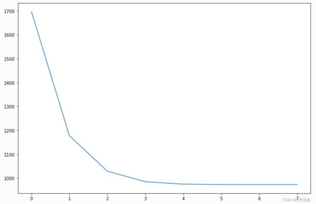
回调

在每次优化迭代期间执行回调。自己编写也很容易。

• deviance - model deviance

• diffs - differences of coefficient norm

• accuracy - model accuracy for LogisticGAM

• coef - coefficient logging

• deviance - 模型偏差（deviance）：用于评估模型与实际观测数据之间的拟合程度。偏差是一种衡量模型对数据拟合好坏的统计量，值越小表示模型拟合得越好。

• diffs - 系数范数差异（differences of coefficient norm）：用于比较模型中不同系数之间的变化。通过计算系数范数的差异，我们可以了解模型在不同特征上的权重变化情况。

• accuracy - LogisticGAM的模型准确度：适用于LogisticGAM（逻辑斯蒂GAM）模型的准确度度量。它衡量模型在分类问题中正确预测的比例，值越高表示模型的准确性越好。

• coef - 系数记录（coefficient logging）：用于记录模型中的系数。通过记录模型的系数，我们可以查看每个特征的权重或影响程度，从而对模型进行解释和理解。系数记录可以帮助我们了解哪些特征对于预测结果的贡献较大或较小。

您可以通过检查以下代码来检查回调：

_ = plt.plot(gam.logs_['deviance'])

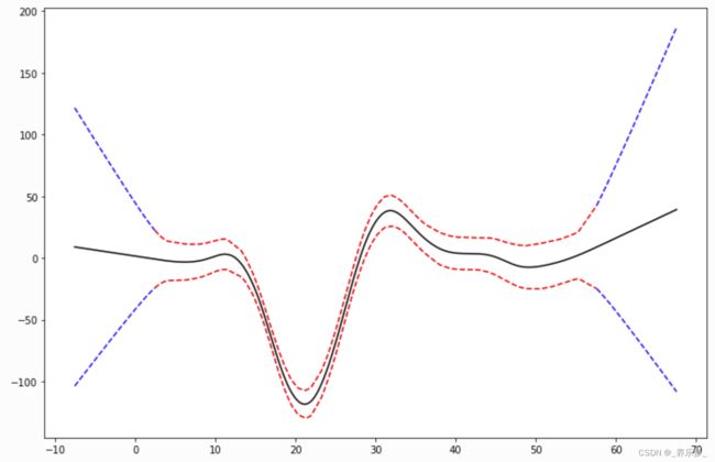
线性外推

from pygam import LinearGAM
from pygam.datasets import mcycle

X, y = mcycle()

gam = LinearGAM()
gam.gridsearch(X, y)

XX = gam.generate_X_grid(term=0)

m = X.min()
M = X.max()
XX = np.linspace(m - 10, M + 10, 500)
Xl = np.linspace(m - 10, m, 50)
Xr = np.linspace(M, M + 10, 50)

plt.figure()

plt.plot(XX, gam.predict(XX), 'k')
plt.plot(Xl, gam.confidence_intervals(Xl), color='b', ls='--')
plt.plot(Xr, gam.confidence_intervals(Xr), color='b', ls='--')
_ = plt.plot(X, gam.confidence_intervals(X), color='r', ls='--')

三、参考

1. Simon N. Wood, 2006
   Generalized Additive Models: an introduction with R

2. Hastie, Tibshirani, Friedman
   The Elements of Statistical Learning
   http://statweb.stanford.edu/~tibs/ElemStatLearn/printings/ESLII_print10.pdf

3. James, Witten, Hastie and Tibshirani
   An Introduction to Statistical Learning
   http://www-bcf.usc.edu/~gareth/ISL/ISLR%20Sixth%20Printing.pdf

4. Paul Eilers & Brian Marx, 1996 Flexible Smoothing with B-splines and Penalties http://www.stat.washington.edu/courses/stat527/s13/readings/EilersMarx_StatSci_1996.pdf

5. Kim Larsen, 2015
   GAM: The Predictive Modeling Silver Bullet
   http://multithreaded.stitchfix.com/assets/files/gam.pdf

6. Deva Ramanan, 2008
   UCI Machine Learning: Notes on IRLS
   http://www.ics.uci.edu/~dramanan/teaching/ics273a_winter08/homework/irls_notes.pdf

7. Paul Eilers & Brian Marx, 2015
   International Biometric Society: A Crash Course on P-splines
   http://www.ibschannel2015.nl/project/userfiles/Crash_course_handout.pdf

8. Keiding, Niels, 1991
   Age-specific incidence and prevalence: a statistical perspective

https://pygam.readthedocs.io/en/latest/notebooks/tour_of_pygam.html

声明：
本人作为一名作者，非常重视自己的作品和知识产权。在此声明，本人的所有原创文章均受版权法保护，未经本人授权，任何人不得擅自公开发布。
本人的文章已经在一些知名平台进行了付费发布，希望各位读者能够尊重知识产权，不要进行侵权行为。任何未经本人授权而将付费文章免费或者付费（包含商用）发布在互联网上的行为，都将视为侵犯本人的版权，本人保留追究法律责任的权利。
谢谢各位读者对本人文章的关注和支持！