目录
- 1 背景
- 2 数据预处理
- 3 需求1:把娱乐/明星八卦单独拉出来
- 3.1 检验一下人数
- 3.2 针对score进行降序排列
- 3.3 看分布
- 3.4 分区间段进行统计人数
- 3.5 直接分成三块
- 3.6 等人数的分块
- 3.7 给这部分进行打标签
- 4 需求2:聚类
- 4.1 先根据娱乐的id将所有含娱乐标签的用户均返回
- 4.2 对反斜杠进行处理
- 4.3 统计2469用户的兴趣点频数
- 4.4 测试迭代器中的组合函数
- 4.5 两两组合
- 5 封装成函数
- 6 单独测试
- 7 进行kmeans聚类
- 7.1 建模
- 7.2 拟合模型
- 7.3 查看拟合结果 即类别标签
- 7.4 将标签放到原数据框
- 7.5 查看聚类中心
- 7.6 可视化展示
- 7.7 算两个变量有一个为0的的个数
背景
现在原始数据是这样:

- 我们希望首先根据score的大小进行某一标签的人群的一个划分
- 其次希望得到不同标签用户之间的相关性,即进行聚类,看含有哪些标签的人群更类似,或者说哪些标签之间会有强相关,进而去进行同步推送相关文章。
数据预处理
读入数据
import pandas as pd
df = pd.read_excel('./example_data.xlsx', sheet_name='Sheet1')
print(df.shape)
df.head()
(37142, 3)
|
device_uuid |
interests_news |
interests_score |
| 0 |
00:08:22:2e:db:fb |
体育 |
0.364912 |
| 1 |
00:08:22:2e:db:fb |
体育/中国足球 |
0.659644 |
| 2 |
00:08:22:2e:db:fb |
体育/乒乓球 |
0.368236 |
| 3 |
00:08:22:2e:db:fb |
健康/养生 |
0.448471 |
| 4 |
00:08:22:2e:db:fb |
娱乐 |
0.263637 |
df['interests_news'].value_counts()
娱乐/明星八卦      2469
社会           1785
娱乐           1582
娱乐/电视         989
娱乐/综艺         935
健康/养生         881
社会/国际         857
社会/民生         747
要闻/国外         705
军事/军情         702
娱乐/电影         653
军事/装备         615
社会/市井         591
情感/两性         523
健康/医疗         513
要闻/国内         491
财经/商业         487
历史/古代史        436
历史/近现代史       428
汽车/用车         417
房产/购房         406
体育/NBA        394
社会/天气         374
体育/中国足球       368
生活/生活常识技巧     357
历史/世界史        354
体育/国际足球       340
手机/安卓         330
军事            296
美食/美食趣闻       288
             ...
数码/配件           3
小品              3
科技/新科技          3
教育/演讲           3
财经/创业           3
房产/政策           2
人工智能            2
财经/基金           2
艺术/歌舞           2
人文/风水命理         2
财经/贵金属          2
财经/债券           2
故事              2
汽车/试驾测评         2
动漫/国产动漫         1
艺术/建筑设计         1
社会/违法犯罪         1
搞笑/创意广告         1
互联网/干货          1
教育/外语           1
艺术/乐器           1
体育/极限运动         1
艺术/戏曲           1
体育/赛车           1
人文/美文           1
科技/人工智能         1
演出现场            1
房产/土地           1
游戏/单机游戏         1
财经/保险           1
Name: interests_news, Length: 224, dtype: int64
删去缺失值
df1 = df.dropna()
print(df1.shape)
df1.head()
(31878, 3)
|
device_uuid |
interests_news |
interests_score |
| 0 |
00:08:22:2e:db:fb |
体育 |
0.364912 |
| 1 |
00:08:22:2e:db:fb |
体育/中国足球 |
0.659644 |
| 2 |
00:08:22:2e:db:fb |
体育/乒乓球 |
0.368236 |
| 3 |
00:08:22:2e:db:fb |
健康/养生 |
0.448471 |
| 4 |
00:08:22:2e:db:fb |
娱乐 |
0.263637 |
需求1:把娱乐/明星八卦单独拉出来
df_yl = df1[df1['interests_news'] == '娱乐/明星八卦']
print(df_yl.shape)
df_yl.head()
(2469, 3)
|
device_uuid |
interests_news |
interests_score |
| 5 |
00:08:22:2e:db:fb |
娱乐/明星八卦 |
0.320401 |
| 14 |
00:08:22:4a:bf:fb |
娱乐/明星八卦 |
0.110526 |
| 36 |
283fd380ea20bdb9 |
娱乐/明星八卦 |
0.546335 |
| 56 |
359168070332202 |
娱乐/明星八卦 |
0.335987 |
| 62 |
38:bc:1a:2f:3d:1c |
娱乐/明星八卦 |
0.244456 |
检验一下人数
len(df_yl['device_uuid'].unique())
2469
针对score进行降序排列
df_yl_sort = df_yl.sort_values(by = 'interests_score', ascending=0)
df_yl_sort.head()
|
device_uuid |
interests_news |
interests_score |
| 16873 |
CQk2NThjZWRjNzUwNzE2NDI3CTc0MUFFQ1FIMjJKVlQ%3D |
娱乐/明星八卦 |
0.994818 |
| 14027 |
CQk1MjQyMjdkYTAyOWJjMjBhCUEwMkFBQ1BTTkJMREo%3D |
娱乐/明星八卦 |
0.980142 |
| 34036 |
CQliMTgyYmYxMzVmNzJjNGM5CTc0MUFFQ1FTMkdWREw%3D |
娱乐/明星八卦 |
0.978786 |
| 8773 |
869322020959563 |
娱乐/明星八卦 |
0.974777 |
| 2967 |
867246026306168 |
娱乐/明星八卦 |
0.973836 |
看分布
import matplotlib
from matplotlib import pyplot as plt
plt.hist(df_yl['interests_score'])
plt.show()
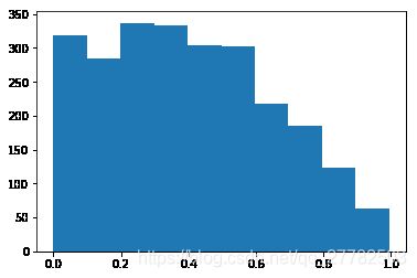
分区间段进行统计人数
pd.cut(df_yl['interests_score'], bins = 5).value_counts()
(0.199, 0.398]        670
(0.398, 0.597]        606
(-0.000971, 0.199]    603
(0.597, 0.796]        403
(0.796, 0.995]        187
Name: interests_score, dtype: int64
直接分成三块
pd.cut(df_yl['interests_score'], bins = 3).value_counts()
(-0.000971, 0.332]    1061
(0.332, 0.663]         968
(0.663, 0.995]         440
Name: interests_score, dtype: int64
等人数的分块
pd.qcut(df_yl['interests_score'], 3).value_counts()
(0.517, 0.995]        823
(0.263, 0.517]        823
(-0.000976, 0.263]    823
Name: interests_score, dtype: int64
总结:
- cut是基于箱子的间隔 区间长度一样 即等区间
- qcut是基于箱子里面的样本量个数分 区间里面样本量一致 即等频数
给这部分进行打标签
df_yl['yl_label'] = pd.cut(df_yl['interests_score'], bins = 3, labels=['低', '中', '高'])
df_yl.head()
|
device_uuid |
interests_news |
interests_score |
yl_label |
| 5 |
00:08:22:2e:db:fb |
娱乐/明星八卦 |
0.320401 |
低 |
| 14 |
00:08:22:4a:bf:fb |
娱乐/明星八卦 |
0.110526 |
低 |
| 36 |
283fd380ea20bdb9 |
娱乐/明星八卦 |
0.546335 |
中 |
| 56 |
359168070332202 |
娱乐/明星八卦 |
0.335987 |
中 |
| 62 |
38:bc:1a:2f:3d:1c |
娱乐/明星八卦 |
0.244456 |
低 |
需求2:聚类
先根据娱乐的id将所有含娱乐标签的用户均返回
yl_list = df1[df1['interests_news'] == '娱乐/明星八卦']['device_uuid'].tolist()
print(len(yl_list))
2469
df1_all = df1[df1['device_uuid'].isin(yl_list)]
print(df1_all.shape)
df1_all.head()
(22399, 3)
|
device_uuid |
interests_news |
interests_score |
| 0 |
00:08:22:2e:db:fb |
体育 |
0.364912 |
| 1 |
00:08:22:2e:db:fb |
体育/中国足球 |
0.659644 |
| 2 |
00:08:22:2e:db:fb |
体育/乒乓球 |
0.368236 |
| 3 |
00:08:22:2e:db:fb |
健康/养生 |
0.448471 |
| 4 |
00:08:22:2e:db:fb |
娱乐 |
0.263637 |
对反斜杠进行处理
遇到的坑:
- 输出文件的路径名称里不能有 | / \
- 控制格式输出的时候 前面必须得是%d %s 啥的 后面是具体的数 不要搞懵逼了
- DataFrame对某一列进行修改的时候 等式左边就把那一列给写上即可 不要就没有保留这个DataFrame
def TransChar(x):
return x.replace('/', '-')
import copy
df1_test = copy.deepcopy(df1_all)
df1_test['interests_news'] = df1_test['interests_news'].map(str).map(TransChar)
df1_all = df1_test
df1_all.head()
|
device_uuid |
interests_news |
interests_score |
| 0 |
00:08:22:2e:db:fb |
体育 |
0.364912 |
| 1 |
00:08:22:2e:db:fb |
体育-中国足球 |
0.659644 |
| 2 |
00:08:22:2e:db:fb |
体育-乒乓球 |
0.368236 |
| 3 |
00:08:22:2e:db:fb |
健康-养生 |
0.448471 |
| 4 |
00:08:22:2e:db:fb |
娱乐 |
0.263637 |
统计2469用户的兴趣点频数
df1_all['interests_news'].value_counts()
娱乐-明星八卦    2469
娱乐         1494
社会         1257
娱乐-综艺       805
娱乐-电视       800
社会-国际       663
娱乐-电影       562
社会-民生       560
社会-市井       485
健康-养生       427
财经-商业       392
情感-两性       351
要闻-国外       335
健康-医疗       332
历史-古代史      315
汽车-用车       307
历史-近现代史     307
军事-装备       274
军事-军情       269
手机-安卓       256
体育-NBA      246
房产-购房       242
美食-美食趣闻     234
体育-国际足球     232
体育-中国足球     231
历史-世界史      230
要闻-国内       220
社会-天气       206
搞笑          189
社会-交通出行     187
           ...
数码-配件         3
科技-新科技        3
音乐-舞蹈         3
娱乐-娱乐资讯       3
小品            3
房产-房企         3
游戏-联机游戏       3
曲艺-杂技         2
舞蹈-广场舞        2
汽车-试驾测评       2
故事            2
财经-基金         2
艺术-歌舞         2
人文-风水命理       2
房产-政策         1
互联网-干货        1
财经-创业         1
搞笑-创意广告       1
艺术-戏曲         1
财经-债券         1
教育-演讲         1
社会-违法犯罪       1
艺术-乐器         1
体育-赛车         1
体育-极限运动       1
人工智能          1
游戏-单机游戏       1
动漫-国产动漫       1
教育-外语         1
演出现场          1
Name: interests_news, Length: 217, dtype: int64
yl_label_all = df1_all['interests_news'].value_counts().reset_index()
yl_label_all = yl_label_all[yl_label_all['interests_news'] > 100]
yl_label_all_list = yl_label_all['index'].tolist()
yl_label_need_list = [x for x in yl_label_all_list if '-' in x]
print(len(yl_label_need_list))
yl_label_need_list
45


['娱乐-明星八卦',
 '娱乐-综艺',
 '娱乐-电视',
 '社会-国际',
 '娱乐-电影',
 '社会-民生',
 '社会-市井',
 '健康-养生',
 '财经-商业',
 '情感-两性',
 '要闻-国外',
 '健康-医疗',
 '历史-古代史',
 '汽车-用车',
 '历史-近现代史',
 '军事-装备',
 '军事-军情',
 '手机-安卓',
 '体育-NBA',
 '房产-购房',
 '美食-美食趣闻',
 '体育-国际足球',
 '体育-中国足球',
 '历史-世界史',
 '要闻-国内',
 '社会-天气',
 '社会-交通出行',
 '时尚-时装',
 '生活-生活常识技巧',
 '汽车-行业',
 '美食-食谱',
 '旅游-美景',
 '育儿-亲子',
 '情感-心理',
 '家居-家装',
 '人文-人文科普',
 '娱乐-音乐',
 '教育-高校',
 '互联网-电商',
 '军事-军人',
 '社会-法制',
 '汽车-新车',
 '体育-CBA',
 '社会-市政基建',
 '财经-股票']
测试迭代器中的组合函数
from itertools import combinations
com_all = list(combinations([1,2,3,4,5], 2))
com_all[0][1]
2
两两组合
from itertools import combinations
com_all = list(combinations(yl_label_need_list, 2))
print(len(com_all))
com_all[0:5]
990


[('娱乐-明星八卦', '娱乐-综艺'),
 ('娱乐-明星八卦', '娱乐-电视'),
 ('娱乐-明星八卦', '社会-国际'),
 ('娱乐-明星八卦', '娱乐-电影'),
 ('娱乐-明星八卦', '社会-民生')]
总结:
- 如果想要实现从一个list中获得所有的两两组合 可以使用combinations函数
封装成函数
df1_all.head()
|
device_uuid |
interests_news |
interests_score |
| 0 |
00:08:22:2e:db:fb |
体育 |
0.632 |
| 1 |
00:08:22:2e:db:fb |
体育-中国足球 |
0.940 |
| 2 |
00:08:22:2e:db:fb |
体育-乒乓球 |
0.975 |
| 3 |
00:08:22:2e:db:fb |
健康-养生 |
0.695 |
| 4 |
00:08:22:2e:db:fb |
娱乐 |
0.655 |
总结遇到的坑:
- 输出文件路径不能有一些特殊的字符 这个得注意 前面也提到过
- 如果老是输出有问题 不要急躁 拿一个小demo出来跑 看看到底是哪一步出了问题 一层一层的去寻找
- 控制格式输出的时候 前面肯定是 %s %d 后面是具体的字母
from sklearn.cluster import KMeans
import pandas as pd
import numpy as np
import matplotlib
from matplotlib import pyplot as plt
import time
def rule(x,y):
if x == 0 or y == 0:
return 1
else:
return 0
def Cluster2(label1, label2):
try:
clus_1 = [label1, label2]
df1_clus_1 = df1_all[df1_all['interests_news'].isin(clus_1)]
print('%s,%s,共有 %s 样本量'% (label1, label2, df1_clus_1.shape[0]))
df1_clus_1.head()
df1_clus_1_ = pd.pivot_table(df1_clus_1,index=["device_uuid"],values=["interests_score"],
columns=["interests_news"],aggfunc=[sum])
df1_clus_1_.head()
df1_clus_1_ = df1_clus_1_.fillna(0)
df1_clus_1_.columns = df1_clus_1_.columns.droplevel()
df1_clus_1_.columns = df1_clus_1_.columns.droplevel()
del df1_clus_1_.columns.name
df1_clus_1_.head()
df1_clus_1_['device_uuid'] = df1_clus_1_.index
df1_clus_1_.head()
df1_clus_1_.index = range(len(df1_clus_1_))
print('数据规整ok之后的样子为')
print(df1_clus_1_.shape)
print(df1_clus_1_.head())
df1_clus_1_['Zero_num'] = df1_clus_1_.apply(lambda x : rule(x[label1], x[label2]), axis=1)
print('两标签任一为0的总人数有: ', df1_clus_1_['Zero_num'].sum())
df1_clus_1_ = df1_clus_1_[df1_clus_1_['Zero_num']!=1]
df1_clus_1_.index = range(len(df1_clus_1_))
print('过滤掉任一为0之后的数据长这样:')
print(df1_clus_1_.shape)
print(df1_clus_1_.head())
estimator = KMeans(n_clusters=2, random_state=23)
estimator.fit(df1_clus_1_.iloc[:,:2])
df1_clus_1_['clu_label'] = estimator.labels_
centroid = estimator.cluster_centers_
print('聚类中心为: ', centroid)
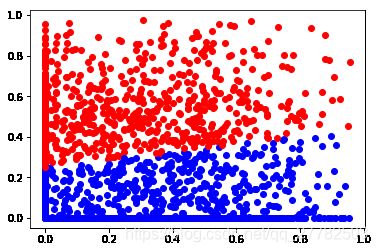
mark = ['or', 'ob']
for i in range(len(df1_clus_1_)):
plt.plot(df1_clus_1_.iloc[i,0], df1_clus_1_.iloc[i,1], mark[estimator.labels_[i]])
plt.show()
plt.close()
return df1_clus_1_
except Exception as e:
print('报错信息为: ', e)
t0 = time.time()
for i in range(len(com_all)):
print('正在输出第 %d 种组合的聚类结果' % (i+1))
print('△'*30)
try:
df1_clus_1_ = Cluster2(com_all[i][0], com_all[i][1])
df1_clus_1_.to_csv('./娱乐大类/[%d]-[%s]_[%s]聚类结果.csv' % (i+1, str(com_all[i][0]), str(com_all[i][1])),
index = False, encoding = 'gbk')
except Exception as e:
print('第 %d 组合的报错信息为: %s' % (i+1, e))
break
t1 = time.time()
print('组合所需时间为:%.2f s' % (t1-t0))
正在输出第 1 种组合的聚类结果
△△△△△△△△△△△△△△△△△△△△△△△△△△△△△△
娱乐-明星八卦,娱乐-综艺,共有 3274 样本量
数据规整ok之后的样子为
(2469, 3)
    娱乐-明星八卦     娱乐-综艺     device_uuid
0  0.875306  0.509272  86164703743646
1  0.469882  0.148727  86164703912396
2  0.077557  0.237983  86168103831042
3  0.203994  0.000000  86168103957564
4  0.001791  0.000000  86185103101184
两标签任一为0的总人数有:  1664
过滤掉任一为0之后的数据长这样:
(805, 4)
    娱乐-明星八卦     娱乐-综艺     device_uuid  Zero_num
0  0.875306  0.509272  86164703743646         0
1  0.469882  0.148727  86164703912396         0
2  0.077557  0.237983  86168103831042         0
3  0.632685  0.092836  86185103874437         0
4  0.158385  0.186337  86208603366335         0
聚类中心为:  [[0.66513518 0.32434565]
 [0.22094246 0.38035482]]
组合所需时间为:2.16 s
单独测试
clus_1 = ['娱乐', '社会']
df1_clus_1 = df1_all[df1_all['interests_news'].isin(clus_1)]
print(df1_clus_1.shape)
df1_clus_1.head()
(2751, 3)
|
device_uuid |
interests_news |
interests_score |
| 4 |
00:08:22:2e:db:fb |
娱乐 |
0.263637 |
| 10 |
00:08:22:2e:db:fb |
社会 |
0.444324 |
| 13 |
00:08:22:4a:bf:fb |
娱乐 |
0.007945 |
| 35 |
283fd380ea20bdb9 |
娱乐 |
0.104760 |
| 44 |
283fd380ea20bdb9 |
社会 |
0.220708 |
根据上表进行透视表操作然后聚类
df1_clus_1_ = pd.pivot_table(df1_clus_1,index=["device_uuid"],values=["interests_score"],
               columns=["interests_news"],aggfunc=[sum])
df1_clus_1_.head()
|
sum |
|
interests_score |
| interests_news |
娱乐 |
社会 |
| device_uuid |
|
|
| 86164703743646 |
0.331710 |
NaN |
| 86164703912396 |
0.034218 |
0.147317 |
| 86168103831042 |
0.197933 |
0.622465 |
| 86185103101184 |
NaN |
0.161907 |
| 86185103527445 |
NaN |
0.546773 |
总结1:
- 使用pandas中的pivot_table函数可以起到和excel透视表一样的功能
- index为根据这个进行分组
- values则是要填充的值为这个
- columns表示列名
- aggfunc为values放进去是怎么放?是sum还是mean还是len
去掉pivot_table之后产生的多重索引的方法:
- 使用columns.droplevel()函数
- 删去列名 columns.name
df1_clus_1_ = df1_clus_1_.fillna(0)
df1_clus_1_.columns = df1_clus_1_.columns.droplevel()
df1_clus_1_.columns = df1_clus_1_.columns.droplevel()
del df1_clus_1_.columns.name
df1_clus_1_.head()
|
娱乐 |
社会 |
| device_uuid |
|
|
| 86164703743646 |
0.331710 |
0.000000 |
| 86164703912396 |
0.034218 |
0.147317 |
| 86168103831042 |
0.197933 |
0.622465 |
| 86185103101184 |
0.000000 |
0.161907 |
| 86185103527445 |
0.000000 |
0.546773 |
df1_clus_1_['device_uuid'] = df1_clus_1_.index
df1_clus_1_.head()
|
娱乐 |
社会 |
device_uuid |
| device_uuid |
|
|
|
| 86164703743646 |
0.331710 |
0.000000 |
86164703743646 |
| 86164703912396 |
0.034218 |
0.147317 |
86164703912396 |
| 86168103831042 |
0.197933 |
0.622465 |
86168103831042 |
| 86185103101184 |
0.000000 |
0.161907 |
86185103101184 |
| 86185103527445 |
0.000000 |
0.546773 |
86185103527445 |
df1_clus_1_.index = range(len(df1_clus_1_))
print(df1_clus_1_.shape)
df1_clus_1_.head()
(1821, 3)
|
娱乐 |
社会 |
device_uuid |
| 0 |
0.331710 |
0.000000 |
86164703743646 |
| 1 |
0.034218 |
0.147317 |
86164703912396 |
| 2 |
0.197933 |
0.622465 |
86168103831042 |
| 3 |
0.000000 |
0.161907 |
86185103101184 |
| 4 |
0.000000 |
0.546773 |
86185103527445 |
进行kmeans聚类
建模
from sklearn.cluster import KMeans
estimator = KMeans(n_clusters=2, random_state=23)
estimator
KMeans(algorithm='auto', copy_x=True, init='k-means++', max_iter=300,
    n_clusters=2, n_init=10, n_jobs=None, precompute_distances='auto',
    random_state=23, tol=0.0001, verbose=0)
拟合模型
df1_clus_1_.iloc[:,:2].head()
|
娱乐 |
社会 |
| 0 |
0.331710 |
0.000000 |
| 1 |
0.034218 |
0.147317 |
| 2 |
0.197933 |
0.622465 |
| 3 |
0.000000 |
0.161907 |
| 4 |
0.000000 |
0.546773 |
estimator.fit(df1_clus_1_.iloc[:,:2])
KMeans(algorithm='auto', copy_x=True, init='k-means++', max_iter=300,
    n_clusters=2, n_init=10, n_jobs=None, precompute_distances='auto',
    random_state=23, tol=0.0001, verbose=0)
查看拟合结果 即类别标签
estimator.labels_
array([1, 1, 0, ..., 1, 1, 1], dtype=int32)
将标签放到原数据框
df1_clus_1_['clu_label'] = estimator.labels_
df1_clus_1_.head()
|
娱乐 |
社会 |
device_uuid |
clu_label |
| 0 |
0.331710 |
0.000000 |
86164703743646 |
1 |
| 1 |
0.034218 |
0.147317 |
86164703912396 |
1 |
| 2 |
0.197933 |
0.622465 |
86168103831042 |
0 |
| 3 |
0.000000 |
0.161907 |
86185103101184 |
1 |
| 4 |
0.000000 |
0.546773 |
86185103527445 |
0 |
df1_clus_1_.iloc[0,0]
0.33171015445836183
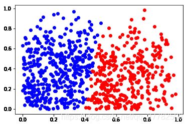
查看聚类中心
centroid = estimator.cluster_centers_
centroid
array([[0.25107961, 0.53625566],
       [0.33770399, 0.07484127]])
可视化展示
mark = ['or', 'ob']
for i in range(len(df1_clus_1_)):
plt.plot(df1_clus_1_.iloc[i,0], df1_clus_1_.iloc[i,1], mark[estimator.labels_[i]])
算两个变量有一个为0的的个数
思路:新增一列 为0的则记为1
def rule(x,y):
    if x == 0 or y == 0:
        return 1
    else:
        return 0
df1_clus_1_['Zero_num'] = df1_clus_1_.apply(lambda x : rule(x['娱乐'], x['社会']), axis=1)
print('两标签任一为0的总人数有: ', df1_clus_1_['Zero_num'].sum())
df1_clus_1_ = df1_clus_1_[df1_clus_1_['Zero_num']!=1]
df1_clus_1_.head()
两标签任一为0的总人数有: 891
|
娱乐 |
社会 |
device_uuid |
clu_label |
Zero_num |
| 1 |
0.034218 |
0.147317 |
86164703912396 |
1 |
0 |
| 2 |
0.197933 |
0.622465 |
86168103831042 |
0 |
0 |
| 7 |
0.077339 |
0.388035 |
86208603366335 |
0 |
0 |
| 10 |
0.402624 |
0.212100 |
86247803073494 |
1 |
0 |
| 11 |
0.237287 |
0.268475 |
86249303752541 |
1 |
0 |
891 / 2751
0.3238822246455834
算两个变量的相关系数
import numpy as np
np.corrcoef(df1_clus_1_['娱乐'], df1_clus_1_['社会'])
array([[ 1.        , -0.02175822],
       [-0.02175822,  1.        ]])
数据
example_data