如何研究带有不可微项的目标函数的局部极小值？

以optimtool的算法为例来解释

在Python >3.7的编程环境下，按如下方式下载optimtool，一个基于符号微分与数值近似的优化方法库：

pip install optimtool --upgrade
pip install optimtool>=2.4.2

目前没有为目标函数中不可微项增加预处理近似，下文介绍了如何通过现有方法研究带不可微项的目标函数的极小值。

常见的不可微项的邻近算子举例

根据文再文的《最优化：建模、算法与理论》的解释，有如下范数或函数的邻近算子（常数$t>0$为正实数）：

• L1范数：
  $$h(x)=||x|{|}_1,pro{x}_{th}(x)=\mathrm{sign}(x)\max \{|x|-t,0\}.$$
• L2范数
  $$h(x)=||x|{|}_2,pro{x}_{th}(x)=\begin{array}{r}(1-\frac{t}{||x|{|}_2})x,||x|{|}_2\ge t\\ 0,其他\end{array}$$
• 二次函数（其中A对称正定）
  $$h(x)=\frac{1}{2}{x}^{T}Ax+b^{T}x+c,pro{x}_{th}(x)=(I+tA{)}^{-1}(x-tb).$$
• 负自然对数的和
  $$h(x)=-\sum _{i=1}^n\ln x_i,pro{x}_{th}(x{)}_i=\frac{x_i+\sqrt{x_i^2+4t}}{2},i=1,2,...,n.$$

以对数罚函数为例来解释算法设计

（对数罚函数）对不等式约束最优化问题，定义对数罚函数：
$$P_I(x,\sigma )=f(x)-\sigma \sum _{i\in \mathcal{I}}\ln (-c_i(x))$$
其中等式右端第二项称为惩罚项，$\sigma >0$称为罚因子。

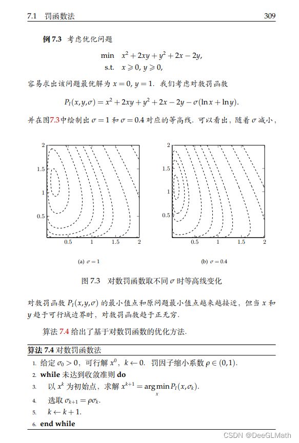
考虑下面这个优化问题（书中第309页）：
$$\begin{gathered} \min x^2+2xy+y^2+2x-2y \\ s.t.x\ge 0,y\ge 0 \end{gathered}$$
通过邻近算子近似的方法来求得目标函数的极小值：

import numpy as np
import sympy as sp
from optimtool._convert import f2m, a2m, p2t # (list or tuple) -> sympy.Matrix
from optimtool._utils import get_value, plot_iteration

DataType = np.float64

def neg_log(funcs, 
			sigma, 
			args, 
			x_0, 
			tk: float=0.02, 
			epsilon: float=1e-10, 
			k: int=0):
	assert tk > 0
	funcs, args, x_0 = f2m(funcs), a2m(args), p2t(x_0)
	res, point = funcs.jacobian(args), []
	while 1:
		reps = dict(zip(args, x_0))
		point.append(x_0)
		grad = np.array(res.subs(reps)).astype(DataType)
		x_0 = ((x_0 - tk * grad[0]) + np.sqrt((x_0 - tk * grad[0])**2 + 4 * tk * sigma)) / 2
		k = k + 1
		if np.linalg.norm(x_0 - point[k - 1]) < epsilon:
			point.append(x_0)
			break
	return x_0, k

def penalty_interior_log(funcs, 
						 args,
						 x_0, 
						 draw: bool=True, 
						 output_f: bool=False, 
						 sigma: int=12, 
						 p: float=0.6, 
						 epsilon: float=1e-10, 
						 k: int=0):
    assert sigma > 0
    assert p > 0
    assert p < 1
    funcs, args, x_0 = f2m(funcs), a2m(args), p2t(x_0)
    point, f = [], [] # 中途点与中途值（由于高维的问题不方便绘制立体图，采用这种方案来反馈优化迭代信息。）
    while 1:
        point.append(np.array(x_0))
        f.append(get_value(funcs, args, x_0))
        x_0, _ = neg_log(funcs, sigma, args, tuple(x_0))
        k = k + 1
        sigma = p * sigma
        if np.linalg.norm(x_0 - point[k - 1]) < epsilon:
            point.append(np.array(x_0))
            f.append(get_value(funcs, args, x_0))
            break
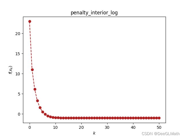
    plot_iteration(f, draw, "penalty_interior_log")
    return (x_0, k, f) if output_f is True else (x_0, k)

示例与邻近算子的可行迭代方案

为了方便表示，我们令$x=x_1$，$y=x_2$，有：
$$\begin{gathered} \min x_1^2+2x_1{x}_2+x_2^2+2x_1-2x_2 \\ s.t.-x_1\le 0,-x_2\le 0 \end{gathered}$$
令$y_1=-(-x_1)$，$y_2=-(-x_2)$，有：
$$y_1=x_1,y_2=x_2$$
即有方程：
$$\begin{gathered} \min y_1^2+2y_1{y}_2+y_2^2+2y_1-2y_2 \\ s.t.y_1\ge 0,y_2\ge 0 \end{gathered}$$
构造如下：

x1, x2 = sp.symbols("x1 x2")
obf = x1**2 + 2*x1*x2 + x2**2 + 2*x1 - 2*x2
print(penalty_interior_log(obf, [x1, x2], (2, 3)))

相比需要修正无穷大值近似的matlab方法，这种方法更加的轻量且数值精度相当地高！！！
结果如下：

(array([0, 1]), 50）

其他不可微项的邻近算子可以通过模仿neg_log来写，例如L1范数的近似为：

x_0 = np.sign(x_0) * np.max(np.abs(x_0) - tk, 0)

L2范数的近似为：

norm = np.linalg.norm(x_0)
x_0 = (1 - tk / norm) * x_0 if norm > tk else 0

二次函数的近似为：

from optimtool._convert import h2h
A = np.array() # need to input: l*l
b = np.array() # need to input: l*1
ita = np.identity(l) + tk * A
ita = h2h(ita) # 可能需要修正矩阵
x_0 = np.linalg.inv(ita) * (x_0 - tk * b)