基于pyspark的个性化电商广告推荐系统
个性化电商广告推荐系统
- 1. 数据介绍
- 2. 项目实现分析
-
- 2.1 数据概况
- 2.2 业务流程
- 3. 预处理behavior_log数据集
-
- 3.1 创建spark session
- 3.2 读取文件并修改schema
- 3.3 查看数据情况
- 3.4 透视表操作
- 3.5 把btag中的操作转化为打分
- 3.6 根据用户对类目偏好打分训练ALS模型
- 3.7 ALS模型预测 初步存储到redis中
- 4. 分析处理raw_sample数据集
-
- 4.1 加载数据并修改schema
- 4.2 查看数据情况
- 4.3 广告展示位进行热度编码
- 4.4 根据时间戳划分数据集
- 5. 分析处理ad_feature数据集
-
- 5.1 加载数据 并添加 schema
- 5.2 查看数据情况
- 5.3 特征选择
- 6. 分析处理user_profile 数据集
-
- 6.1 加载数据 并添加 schema
- 6.2 查看数据情况
- 6.3 缺失值处理
-
- 6.3.1 利用随机森林对缺失值进行预测
- 6.3.2 缺失值拼接
- 6.3.3 低维转高维方式 缺失项也当做一个单独的特征来对待
- 6.3.4 用户特征合并
- 6.3.5 注意热编码中特征对应关系:
- 7. LR实现CTR估计
-
- 7.1 Spark逻辑回归(LR)模型使用介绍
- 7.2 数据合并、特征组合
- 7.3 划分数据集
- 7.4 创建逻辑回归训练器CTR_Normal,并训练
- 7.5 训练 CTRModel_AllOneHot
- 8. 离线数据缓存之离线召回集
-
- 8.1 ALS模型召回的是用户喜欢的类别,需要通过类别找到对应广告
- 8.2 利用ALS模型进行类别的召回,从而选择商品
- 8.3 只考虑离线的话
- 9. 实时产生推荐结果
-
- 9.1 缓存用户和商品特征
- 9.2 商品特征对应关系
- 9.3 特征获取
- 9.4 载入模型并排序
- 9.5 查看结果
1. 数据介绍
- 原始样本骨架raw_sample
| 字段名 | 解释 |
|---|---|
| user_id | 脱敏过的用户ID |
| adgroup_id | 脱敏过的广告单元ID |
| time_stamp | 时间戳 |
| pid | 资源位 |
| noclk | 为1表示没有点击,为0代表点击 |
| clk | 为0表示没有点击,为1代表点击 |
-
统计点和不点 需要曝光的(所有展示的物品) 和点击的(点击的物品)
-
不能看作分类的结果 因为大多数都是不点的 数值为0
- 最小的不点的值 是0.87 点的概率 0.13 推荐点的概率大的那个
- 广告基本信息表ad_feature
| 字段名 | 解释 |
|---|---|
| adgroup_id | 脱敏过的广告单元ID |
| cate_id | 脱敏过的商品类目ID |
| campaign_id | 脱敏过的广告计划ID |
| customer_id | 脱敏过的广告主ID |
| brand_id | 脱敏过的品牌ID |
| price | 宝贝的价格 |
其中一个广告ID对应一个商品(宝贝),一个宝贝属于一个类目,一个宝贝属于一个品牌。
- 用户基本信息表user_profile
| 字段名 | 解释 |
|---|---|
| userid | 脱敏过的用户ID |
| cms_segid | 微群ID |
| cms_group_id | 微组ID |
| final_gender_code | 性别 1:男 0:女 |
| age_level | 年龄层次 1、2、3、4、5、6、7 |
| pvalue_level | 消费档次 1:低档 2:中档 3:高档 |
| shopping_level | 购物深度 1:浅层用户 2:中度用户 3:深度用户 |
| occupation | 是否大学生 1: 是 0: 否 |
| new_user_class_level | 城市层级 1、2、3、4 |
- 用户的行为日志behavior_log
| 字段名 | 解释 |
|---|---|
| user | 脱敏过的用户ID |
| time_stamp | 时间戳 |
| tag | 行为类型:(类型 | 说明) pv|浏览 cart|加入购物车 fav|喜爱 buy|购买 |
| cate_id | 脱敏过的商品类目ID |
| brand_id | 脱敏过的品牌ID |
2. 项目实现分析
2.1 数据概况
- 一份广告点击的样本数据raw_sample.csv:体现的是用户对不同位置广告点击、没点击的情况
- 一份广告基本信息数据ad_feature.csv:体现的是每个广告的类目(id)、品牌(id)、价格特征
- 一份用户基本信息数据user_profile.csv:体现的是用户群组、性别、年龄、消费购物档次、所在城市级别等特征
- 一份用户行为日志数据behavior_log.csv:体现用户对**商品类目(id)、品牌(id)**的浏览、加购物车、收藏、购买等信息
2.2 业务流程
推荐业务处理主要流程: 召回 ==> 排序 ==> 过滤
- 离线处理业务流
- raw_sample.csv ==> 历史样本数据
- ad_feature.csv ==> 广告特征数据
- user_profile.csv ==> 用户特征数据
- raw_sample.csv + ad_feature.csv + user_profile.csv ==> CTR点击率预测模型
- behavior_log.csv ==> 评分数据 ==> user-cate/brand评分数据 ==> 协同过滤 ==> top-N cate/brand ==> 关联广告
- 协同过滤召回 ==> top-N cate/brand ==> 关联对应的广告完成召回
- 在线处理业务流
- 数据处理部分:
- 实时行为日志 ==> 实时特征 ==> 缓存
- 实时行为日志 ==> 实时商品类别/品牌 ==> 实时广告召回集 ==> 缓存
- 推荐任务部分:
- CTR点击率预测模型 + 广告/用户特征(缓存) + 对应的召回集(缓存) ==> 点击率排序 ==> top-N 广告推荐结果
- 数据处理部分:
- 因为数据大部分都是不点击, 样本极度偏斜的,点击样本很少 (5%) 预测出的结果都是0 不点
- 根据不点击的概率来排序 不点击概率越低的排在前面
- 在测试数据中 按照不点击的概率排序 考察精准率(找前10个 看看10个中是否有点击的样本)
3. 预处理behavior_log数据集
3.1 创建spark session
import os
# 配置spark driver和pyspark运行时,所使用的python解释器路径
PYSPARK_PYTHON = "/home/hadoop/miniconda3/envs/datapy365spark23/bin/python"
JAVA_HOME='/home/hadoop/app/jdk1.8.0_191'
# 当存在多个版本时,不指定很可能会导致出错
os.environ["PYSPARK_PYTHON"] = PYSPARK_PYTHON
os.environ["PYSPARK_DRIVER_PYTHON"] = PYSPARK_PYTHON
os.environ['JAVA_HOME']=JAVA_HOME
# spark配置信息

from pyspark import SparkConf
from pyspark.sql import SparkSession

SPARK_APP_NMAE = 'preprocessingBehaviorLog'
SPARK_URL = 'spark://192.168.199.188:7077'

conf = SparkConf()
 '''
 创建spark config对象:
 	设置启动的spark的app名称,没有提供,将随机产生一个名称
 	设置spark master的地址
 	设置该app启动时占用的内存用量,默认1g
 	设置spark executor使用的CPU核心数
 '''
config = (
	("spark.app.name",SPARK_APP_NAME),
	("spark.master",SPARK_URL),
	("spark.executor.memory","6g"),
	("spark.executor.cores","4") ,
)
conf.setAll(config)

# 利用config对象,创建spark session
spark = SparkSession.builder.config(conf = conf).getOrCreate()
3.2 读取文件并修改schema
from pyspark.sql.types import *

scheme = StructType([
	StructField("userId",IntegerType()),
  StructField("timestamp",LongType()),
  StructField("btag",StringType()),
  StructField("cateId",IntergerType()),
  StructField("barndId",IntergerType())
])

behavior_log_df = spark.read.csv("datasets/behavior_log.csv",header=True,schema = schema)
behavior_log_df.show()
结果:
+------+----------+----+------+-------+
|userId| timestamp|btag|cateId|brandId|
+------+----------+----+------+-------+
|558157|1493741625|  pv|  6250|  91286|
|558157|1493741626|  pv|  6250|  91286|
|558157|1493741627|  pv|  6250|  91286|
|728690|1493776998|  pv| 11800|  62353|
|332634|1493809895|  pv|  1101| 365477|
|857237|1493816945|  pv|  1043| 110616|
|991528|1493780765|  pv|  7270| 274795|
|991528|1493780764|  pv|  7270| 274795|
|991528|1493780633|  pv|  7270| 274795|
|991528|1493780764|  pv|  7270| 274795|
+------+----------+----+------+-------+
only showing top 20 rows

root
 |-- userId: integer (nullable = true)
 |-- timestamp: long (nullable = true)
 |-- btag: string (nullable = true)
 |-- cateId: integer (nullable = true)
 |-- brandId: integer (nullable = true)
3.3 查看数据情况
'''
  注意 第一个count后返回的是一个dataframe 还没有开始计算
  当调用df.count()时才开始计算,这里count计算的是userId的个数
  collect 会把计算结果全部加在到内存中 这里只有四种类型 谨慎使用
'''
print("查看userId的数据情况: ",behavior_log_df.groupBy('userId').count().count())
print("查看btag的数据情况: ",behavior_log_df.groupBy('btag').count().collect()
print("查看cateId的数据情况:", behavior_log_df.groupBy("cateId").count().count())
print("查看brandId的数据情况:", behavior_log_df.groupBy("brandId").count().count())
print("判断数据是否有空值:",behavior_log_df.count(),behavior_log_df.dropna().count())
结果:
查看user的数据情况: 1136340
查看btag的数据情况: [Row(btag='buy', count=9115919), Row(btag='fav', count=9301837), Row(btag='cart', count=15946033), Row(btag='pv', count=688904345)]
查看cateId的数据情况: 12968
查看brandId的数据情况: 460561
判断数据是否有空值: 723268134 723268134
3.4 透视表操作
'''
	统计每个用户 对 各类商品 的pv、fav、cart、buy数量并转换
	pivot的第二个参数 可以对该标签内的内容排序
	并记录
'''
cate_count_df = behavior_log_df.groupby('userId','cateId').pivot('btag',['pv','fav','cart','buy']).show()

cate_count_df.write.csv("dataset/cate_count.csv", header=True)
3.5 把btag中的操作转化为打分
def process_row(r):
  '''
  把dataframe转换成rdd,每一行应用这个函数
  m: 用户对应的行为次数
  该偏好权重比例,次数上限仅供参考,具体数值应根据产品业务场景权衡
	pv: if m<=20: score=0.2*m; else score=4
	fav: if m<=20: score=0.4*m; else score=8
	cart: if m<=20: score=0.6*m; else score=12
	buy: if m<=20: score=1*m; else score=20
  '''
  pv_count = r.pv if r.pv else 0.0
  fav_count = r.fav if r.fav else 0.0
  cart_count = r.cart if r.cart else 0.0
  buy_count = r.buy if r.buy else 0.0

  pv_score = pv_count*0.2 if pv_count <= 20 else 4.0
  fav_score = 0.4*fav_count if fav_count<=20 else 8.0
  cart_score = 0.6*cart_count if cart_count<=20 else 12.0
  buy_score = 1.0*buy_count if buy_count<=20 else 20.0

  rating = pv_score + fav_score + cart_score + buy_score

  return r.userId,r.cateId,rating

# 注意:toDF不是每个rdd都有的方法,仅局限于此处的rdd
cate_rating_df = cate_count_df.rdd.map(precess_row).toDF(['userId','cateId','rating'])

cate_rating_df
# DataFrame[userId: bigint, cateId: bigint, rating: double]
3.6 根据用户对类目偏好打分训练ALS模型
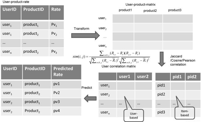
- 通常如果USER-ITEM打分数据应该是通过以下方式进行处理转换为USER-ITEM-MATRIX
'''
任意的聚合函数都可以 只要取得到值 可通过该方法获得 user-cate-matrix
但由于cateId字段过多,这里运算量比很大,机器内存要求很高才能执行,否则无法完成任务
好在我们训练ALS模型时,不需要转换为user-cate-matrix,所以这里可以不用运行
'''
cate_rating_df.groupBy('userId').povit('cateId').min('rating')
- 基于Spark的ALS隐因子模型进行CF评分预测
- ALS的意思是交替最小二乘法(Alternating Least Squares),是Spark2.*中加入的进行基于模型的协同过滤(model-based CF)的推荐系统算法。
- 同SVD,它也是一种矩阵分解技术,对数据进行降维处理。
'''
spark ml的模型训练是基于内存的,如果数据过大,内存空间小,迭代次数过多,可能会造成内存溢出,报错.

设置Checkpoint的话,会把所有数据落盘,这样如果异常退出,下次重启后,可以接着上次的训练节点继续运行,但该方法其实指标不治本,因为无法防止内存溢出,所以还是会报错

如果数据量大,应考虑的是增加内存、或限制迭代次数和训练数据量级等

pysaprk中ml库处理的都是dataframe对象
pysaprk中mllib库处理的都是rdd对象 现在已经不维护 但还能使用

checkPointInterval:每执行几步落盘
存储
'''
from pyspark.ml.recommendation import ALS

spark.sparkContext.setCheckpointDir("hdfs://localhost:8020/checkPoint/")
als = ALS(userCol='userId',itemCol='cateId',ratingCol='rating',checkPointInterval=5)
model = als.fit(cate_rating_df)
model.save("models/userCateRatingALSModel.obj")

'''
加载保存的模型
'''
from pyspark.ml.recommendation import ALSModel
als_model = ALSModel.load("models/userCateRatingALSModel.obj")
3.7 ALS模型预测 初步存储到redis中
'''
model.recommendForAllUsers(N) 给所有用户推荐Top-N个物品
推荐结果保存在recommendation列中
'''
ret = model.recommendForAllUsers(3)
ret2 = model.recommendForAllItems(3)
ret.show()
结果:
+------+--------------------+
|userId|     recommendations|
+------+--------------------+
|   148|[[3347, 12.547271...|
|   463|[[1610, 9.250818]...|
|   471|[[1610, 10.246621...|
|   496|[[1610, 5.162216]...|
|   833|[[5607, 9.065482]...|
|  1088|[[104, 6.886987],...|
|  1238|[[5631, 14.51981]...|
|  1342|[[5720, 10.89842]...|
|  1580|[[5731, 8.466453]...|
+------+--------------------+
初步召回到redis
'''
对每个分片的数据进行处理 mapPartition Transformation   map
foreachPartition Action操作   foreachRDD
一块一块处理 避免频繁的建立断开链接
'''
import redis
host = "192.168.19.8"
port = 6379
def recall_cate_by_cf(partition):
    # 建立redis 连接池
    pool = redis.ConnectionPool(host=host, port=port)
    # 建立redis客户端
    client = redis.Redis(connection_pool=pool)
    for row in partition:
        client.hset("recall_cate", row.userId, [i.cateId for i in row.recommendations])

ret.foreachPartition(recall_cate_by_cf)
4. 分析处理raw_sample数据集
4.1 加载数据并修改schema
'''
使用dataframe.withColumn更改df列数据结构
使用dataframe.withColumnRenamed更改列名称
'''
from pyspark.sql.types import StructType, StructField, IntegerType, StringType, LongType, FloatType

df = spark.read.csv("/datasets/raw_sample.csv",header=True)
raw_sample = df.withColumn('user',df.user.cast(IntergerType())).withColumnRenamed('user','userId').
withColumn('time_stamp',df.time_stamp.cast(LongType())).withColumnRenamed('time_stamp','timestamp').
withColumn("adgroup_id",df.adgroup_id.cast(IntegerType())).withColumnRenamed("adgroup_id", "adgroupId").
withColumn("pid", df.pid.cast(StringType())).
withColumn("nonclk", df.nonclk.cast(IntegerType())).
withColumn("clk", df.clk.cast(IntegerType()))

raw_sample_df.printSchema()
raw_sample_df.show()
结果:
root
 |-- userId: integer (nullable = true)
 |-- timestamp: long (nullable = true)
 |-- adgroupId: integer (nullable = true)
 |-- pid: string (nullable = true)
 |-- nonclk: integer (nullable = true)
 |-- clk: integer (nullable = true)

+------+----------+---------+-----------+------+---+
|userId| timestamp|adgroupId|        pid|nonclk|clk|
+------+----------+---------+-----------+------+---+
|581738|1494137644|        1|430548_1007|     1|  0|
|449818|1494638778|        3|430548_1007|     1|  0|
|914836|1494650879|        4|430548_1007|     1|  0|
|914836|1494651029|        5|430548_1007|     1|  0|
|399907|1494302958|        8|430548_1007|     1|  0|
|628137|1494524935|        9|430548_1007|     1|  0|
|298139|1494462593|        9|430539_1007|     1|  0|
|775475|1494561036|        9|430548_1007|     1|  0|
|555266|1494307136|       11|430539_1007|     1|  0|
|117840|1494036743|       11|430548_1007|     1|  0|
+------+----------+---------+-----------+------+---+
4.2 查看数据情况
print("样本数据集总条目数:", raw_sample_df.count())
print("用户user总数:", raw_sample_df.groupBy("user").count().count())
print("广告id adgroup_id总数:", raw_sample_df.groupBy("adgroup_id").count().count())
print("广告展示位pid情况:", raw_sample_df.groupBy("pid").count().collect())
print("广告点击数据情况clk:", raw_sample_df.groupBy("clk").count().collect())
结果:
样本数据集总条目数: 26557961
用户user总数: 1141729
广告id adgroup_id总数: 846811
广告展示位pid情况: [Row(pid='430548_1007', count=16472898), Row(pid='430539_1007', count=10085063)]
广告点击数据情况clk: [Row(clk='0', count=25191905), Row(clk='1', count=1366056)]
4.3 广告展示位进行热度编码
热独编码 OneHotEncode
-
热独编码是一种经典编码,是使用N位状态寄存器(如0和1)来对N个状态进行编码,每个状态都由他独立的寄存器位,并且在任意时候,其中只有一位有效。
-
假设有三组特征,分别表示年龄,城市,设备;
[“男”, “女”][0,1]
[“北京”, “上海”, “广州”][0,1,2]
[“苹果”, “小米”, “华为”, “微软”][0,1,2,3]
传统变化: 对每一组特征,使用枚举类型,从0开始;
["男“,”上海“,”小米“]=[ 0,1,1]
["女“,”北京“,”微软“] =[1,0,3]
传统变化后的数据不是连续的,而是随机分配的,不容易应用在分类器中
而经过热独编码,数据会变成稀疏的,方便分类器处理:
["男“,”上海“,”小米“]=[ 1,0,0,1,0,0,1,0,0]
["女“,”北京“,”微软“] =[0,1,1,0,0,0,0,0,1]
这样做保留了特征的多样性,但是也要注意如果数据过于稀疏(样本较少、维度过高),其效果反而会变差
-
热编码只能对字符串类型的列数据进行处理
处理流程
-
StringIndexer:对指定字符串列数据进行特征处理,如将性别数据“男”、“女”转化为0和1
OneHotEncoder:对特征列数据,进行热编码,通常需结合StringIndexer一起使用
Pipeline:让数据按顺序依次被处理,将前一次的处理结果作为下一次的输入
from pyspark.ml.feature import StringIndexer
from pyspark.ml.feature import OneHotEncoder
from pyspark.ml import Pipeline

stringindexer = StringIndexer(inputCol='pid',outputCol='pid_feature')
encoder = OneHotEncoder(dropLast='false',inputCol='pid_feature',outputCol='pid_value')
pipeline = Pipeline(stages=[stringindexer,encoder])

pipeline_model = pipeline.fit(raw_sample_df)
new_df = pipeline_model.transform(raw_sample_df)
new_df.show()
结果:
+------+----------+---------+-----------+------+---+-----------+-------------+
|userId| timestamp|adgroupId|        pid|nonclk|clk|pid_feature|    pid_value|
+------+----------+---------+-----------+------+---+-----------+-------------+
|581738|1494137644|        1|430548_1007|     1|  0|        0.0|(2,[0],[1.0])|
|449818|1494638778|        3|430548_1007|     1|  0|        0.0|(2,[0],[1.0])|
|914836|1494650879|        4|430548_1007|     1|  0|        0.0|(2,[0],[1.0])|
|914836|1494651029|        5|430548_1007|     1|  0|        0.0|(2,[0],[1.0])|
|399907|1494302958|        8|430548_1007|     1|  0|        0.0|(2,[0],[1.0])|
|628137|1494524935|        9|430548_1007|     1|  0|        0.0|(2,[0],[1.0])|
|298139|1494462593|        9|430539_1007|     1|  0|        1.0|(2,[1],[1.0])|
|775475|1494561036|        9|430548_1007|     1|  0|        0.0|(2,[0],[1.0])|
|555266|1494307136|       11|430539_1007|     1|  0|        1.0|(2,[1],[1.0])|
|117840|1494036743|       11|430548_1007|     1|  0|        0.0|(2,[0],[1.0])|
|707120|1494220810|       13|430548_1007|     1|  0|        0.0|(2,[0],[1.0])|
|530454|1494293746|       13|430548_1007|     1|  0|        0.0|(2,[0],[1.0])|
+------+----------+---------+-----------+------+---+-----------+-------------+
only showing top 20 rows
pid_value是一个系数向量类型数据SparseVector
from pyspark.ml.linalg import SparseVector
print(SparseVector(4, [1, 3], [3.0, 4.0]))
print(SparseVector(4, [1, 3], [3.0, 4.0]).toArray())
print("*********")
print(new_df.select("pid_value").first())
print(new_df.select("pid_value").first().pid_value.toArray())
结果:
(4,[1,3],[3.0,4.0])
[0. 3. 0. 4.]
*********
Row(pid_value=SparseVector(2, {0: 1.0}))
[1. 0.]
4.4 根据时间戳划分数据集
new_df.sort("timestamp", ascending=False).show()
结果:
+------+----------+---------+-----------+------+---+-----------+-------------+
|userId| timestamp|adgroupId|        pid|nonclk|clk|pid_feature|    pid_value|
+------+----------+---------+-----------+------+---+-----------+-------------+
|177002|1494691186|   593001|430548_1007|     1|  0|        0.0|(2,[0],[1.0])|
|243671|1494691186|   600195|430548_1007|     1|  0|        0.0|(2,[0],[1.0])|
|488527|1494691184|   494312|430548_1007|     1|  0|        0.0|(2,[0],[1.0])|
|488527|1494691184|   431082|430548_1007|     1|  0|        0.0|(2,[0],[1.0])|
| 17054|1494691184|   742741|430548_1007|     1|  0|        0.0|(2,[0],[1.0])|
| 17054|1494691184|   756665|430548_1007|     1|  0|        0.0|(2,[0],[1.0])|
|488527|1494691184|   687854|430548_1007|     1|  0|        0.0|(2,[0],[1.0])|
+------+----------+---------+-----------+------+---+-----------+-------------+
- 本样本数据集为 8天数据
- 前7天为训练数据 后1天为测试
train_sample = raw_sample_df.filter(raw_sample_df.timestamp <= (1494691186-24*60*60))
test_sample = raw_sample_df.filter(raw_sample_df.timestamp>(1494691186-24*60*60))
5. 分析处理ad_feature数据集
5.1 加载数据 并添加 schema
df = spark.read.csv("datasets/ad_feature.csv", header=True)
df.show()    # 展示数据,默认前20条
结果
+----------+-------+-----------+--------+------+-----+
|adgroup_id|cate_id|campaign_id|customer| brand|price|
+----------+-------+-----------+--------+------+-----+
|     63133|   6406|      83237|       1| 95471|170.0|
|    313401|   6406|      83237|       1| 87331|199.0|
|    248909|    392|      83237|       1| 32233| 38.0|
|    208458|    392|      83237|       1|174374|139.0|
|    110847|   7211|     135256|       2|145952|32.99|
|    607788|   6261|     387991|       6|207800|199.0|
|    375706|   4520|     387991|       6|  NULL| 99.0|
|     11115|   7213|     139747|       9|186847| 33.0|
|     24484|   7207|     139744|       9|186847| 19.0|
|     28589|   5953|     395195|      13|  NULL|428.0|
+----------+-------+-----------+--------+------+-----+
- 由于本数据集中存在NULL字样的数据,无法直接设置schema,只能先将NULL类型的数据处理掉,然后进行类型转换
from pyspark.sql.types import StructType, StructField, IntegerType, FloatType

df.replace('NULL','-1')

ad_feature_df = df.withColumn('adgroup_id',df.adgroup_id.cast(IntegerType())).withColumnRenamed('adgroup_id','adgroupId').
withColumn("cate_id", df.cate_id.cast(IntegerType())).withColumnRenamed("cate_id", "cateId").
withColumn("campaign_id",df.campaign_id.cast(IntegerType())).withColumnRenamed("campaign_id", "campaignId").
withColumn("customer", df.customer.cast(IntegerType())).withColumnRenamed("customer", "customerId").
withColumn("brand", df.brand.cast(IntegerType())).withColumnRenamed("brand", "brandId").
withColumn("price", df.price.cast(FloatType()))

ad_feature_df.show()
结果:
+---------+------+----------+----------+-------+-----+
|adgroupId|cateId|campaignId|customerId|brandId|price|
+---------+------+----------+----------+-------+-----+
|    63133|  6406|     83237|         1|  95471|170.0|
|   313401|  6406|     83237|         1|  87331|199.0|
|   248909|   392|     83237|         1|  32233| 38.0|
|   208458|   392|     83237|         1| 174374|139.0|
|   110847|  7211|    135256|         2| 145952|32.99|
|   607788|  6261|    387991|         6| 207800|199.0|
|   375706|  4520|    387991|         6|     -1| 99.0|
|    11115|  7213|    139747|         9| 186847| 33.0|
|    24484|  7207|    139744|         9| 186847| 19.0|
|    28589|  5953|    395195|        13|     -1|428.0|
+---------+------+----------+----------+-------+-----+
5.2 查看数据情况
print("总广告条数:",df.count())   # 数据条数
print("cateId数值个数:", ad_feature_df.groupBy("cateId").count().count())
print("campaignId数值个数:", ad_feature_df.groupBy("campaignId").count().count())
print("customerId数值个数:", ad_feature_df.groupBy("customerId").count().count())
print("brandId数值个数:", ad_feature_df.groupBy("brandId").count().count())
ad_feature_df.sort("price",ascending=False).show()
结果
总广告条数: 846811
cateId数值个数: 6769
campaignId数值个数: 423436
customerId数值个数: 255875
brandId数值个数: 99815
+---------+------+----------+----------+-------+-----+
|adgroupId|cateId|campaignId|customerId|brandId|price|
+---------+------+----------+----------+-------+-----+
|   485749|  9970|    352666|    140520|     -1| 0.01|
|    88975|  9996|    198424|    182415|     -1| 0.01|
|   109704| 10539|     59774|     90351| 202710| 0.01|
|    49911|  7032|    129079|    172334|     -1| 0.01|
|   339334|  9994|    310408|    211292| 383023| 0.01|
|     6636|  6703|    392038|     46239| 406713| 0.01|
|    92241|  6130|     72781|    149714|     -1| 0.01|
+---------+------+----------+----------+-------+-----+
5.3 特征选择
特征选择
- cateId:脱敏过的商品类目ID;
- campaignId:脱敏过的广告计划ID;
- customerId:脱敏过的广告主ID;
- brandId:脱敏过的品牌ID;
以上四个特征均属于分类特征,但由于分类值个数均过于庞大,如果去做热独编码处理,会导致数据过于稀疏 且当前我们缺少对这些特征更加具体的信息,从而无法对这些特征的数据做聚类、降维处理 因此这里不选取它们作为特征
而只选取price作为特征数据,因为价格本身是一个统计类型连续数值型数据,且能很好的体现广告的价值属性特征,通常也不需要做其他处理(离散化、归一化、标准化等),所以这里直接将当做特征数据来使用
6. 分析处理user_profile 数据集
6.1 加载数据 并添加 schema
from pyspark.sql.types import StructType, StructField, StringType, IntegerType, LongType, FloatType

schema = StructType([
    StructField("userId", IntegerType()),
    StructField("cms_segid", IntegerType()),
    StructField("cms_group_id", IntegerType()),
    StructField("final_gender_code", IntegerType()),
    StructField("age_level", IntegerType()),
    StructField("pvalue_level", IntegerType()),
    StructField("shopping_level", IntegerType()),
    StructField("occupation", IntegerType()),
    StructField("new_user_class_level", IntegerType())
])
user_profile_df = spark.read.csv("hdfs://localhost:8020/csv/user_profile.csv", header=True, schema=schema)

user_profile_df.show()
结果
root
 |-- userId: integer (nullable = true)
 |-- cms_segid: integer (nullable = true)
 |-- cms_group_id: integer (nullable = true)
 |-- final_gender_code: integer (nullable = true)
 |-- age_level: integer (nullable = true)
 |-- pvalue_level: integer (nullable = true)
 |-- shopping_level: integer (nullable = true)
 |-- occupation: integer (nullable = true)
 |-- new_user_class_level: integer (nullable = true)

+------+---------+------------+-----------------+---------+------------+--------------+----------+--------------------+
|userId|cms_segid|cms_group_id|final_gender_code|age_level|pvalue_level|shopping_level|occupation|new_user_class_level|
+------+---------+------------+-----------------+---------+------------+--------------+----------+--------------------+
|   234|        0|           5|                2|        5|        null|             3|         0|                   3|
|   523|        5|           2|                2|        2|           1|             3|         1|                   2|
|   612|        0|           8|                1|        2|           2|             3|         0|                null|
|  1670|        0|           4|                2|        4|        null|             1|         0|                null|
|  2545|        0|          10|                1|        4|        null|             3|         0|                null|
|  3644|       49|           6|                2|        6|           2|             3|         0|                   2|
|  5777|       44|           5|                2|        5|           2|             3|         0|                   2|
|  6211|        0|           9|                1|        3|        null|             3|         0|                   2|
|  6355|        2|           1|                2|        1|           1|             3|         0|                   4|
|  6823|       43|           5|                2|        5|           2|             3|         0|                   1|
| 10912|        0|           4|                2|        4|           2|             3|         0|                null|
| 10996|        0|           5|                2|        5|        null|             3|         0|                   4|
| 11256|        8|           2|                2|        2|           1|             3|         0|                   3|
| 11310|       31|           4|                2|        4|           1|             3|         0|                   4|
+------+---------+------------+-----------------+---------+------------+--------------+----------+--------------------+
only showing top 20 rows
6.2 查看数据情况
print("分类特征值个数情况: ")
print("cms_segid: ", user_profile_df.groupBy("cms_segid").count().count())
print("cms_group_id: ", user_profile_df.groupBy("cms_group_id").count().count())
print("final_gender_code: ", user_profile_df.groupBy("final_gender_code").count().count())
print("age_level: ", user_profile_df.groupBy("age_level").count().count())
print("shopping_level: ", user_profile_df.groupBy("shopping_level").count().count())
print("occupation: ", user_profile_df.groupBy("occupation").count().count())

print("含缺失值的特征情况: ")
user_profile_df.groupBy("pvalue_level").count().show()
user_profile_df.groupBy("new_user_class_level").count().show()

t_count = user_profile_df.count()

pl_na_count = t_count - user_profile_df.dropna(subset=["pvalue_level"]).count()
print("pvalue_level的空值情况:", pl_na_count, "空值占比:%0.2f%%"%(pl_na_count/t_count*100))

nul_na_count = t_count - user_profile_df.dropna(subset=["new_user_class_level"]).count()
print("new_user_class_level的空值情况:", nul_na_count, "空值占比:%0.2f%%"%(nul_na_count/t_count*100))
结果
分类特征值个数情况:
cms_segid:  97
cms_group_id:  13
final_gender_code:  2
age_level:  7
shopping_level:  3
occupation:  2
含缺失值的特征情况:
+------------+------+
|pvalue_level| count|
+------------+------+
|        null|575917|
|           1|154436|
|           3| 37759|
|           2|293656|
+------------+------+

+--------------------+------+
|new_user_class_level| count|
+--------------------+------+
|                null|344920|
|                   1| 80548|
|                   3|173047|
|                   4|138833|
|                   2|324420|
+--------------------+------+

pvalue_level的空值情况: 575917 空值占比:54.24%
new_user_class_level的空值情况: 344920 空值占比:32.49%
6.3 缺失值处理
-
注意,一般情况下:
- 缺失率低于10%:可直接进行相应的填充,如默认值、均值、算法拟合等等;
- 高于10%:往往会考虑舍弃该特征
- 特征处理,如1维转多维
-
但根据我们的经验,我们的广告推荐其实和用户的消费水平、用户所在城市等级都有比较大的关联,因此在这里pvalue_level、new_user_class_level都是比较重要的特征,我们不考虑舍弃
-
缺失值处理方案:
- 填充方案:结合用户的其他特征值,利用随机森林算法进行预测;但产生了大量人为构建的数据,一定程度上增加了数据的噪音
- 把变量映射到高维空间:如pvalue_level的1维数据,转换成是否1、是否2、是否3、是否缺失的4维数据;这样保证了所有原始数据不变,同时能提高精确度,但这样会导致数据变得比较稀疏,如果样本量很小,反而会导致样本效果较差,因此也不能滥用
6.3.1 利用随机森林对缺失值进行预测
-
在随机森林中需要用到LabeledPoint
-
对于多类分类,标签应该是从零开始的类索引:0, 1, 2, …
-
第一个参数是目标值,后一个是特征值
-
与我们数据集中从1开始不同,注意转换
-
from pyspark.ml.linalg import SparseVector
from pyspark.mllib.regression import LabeledPoint
pos = LabeledPoint(1.0, [1.0, 0.0, 3.0])
neg = LabeledPoint(0.0, SparseVector(3, [0, 2], [1.0, 3.0]))
-
-
利用随机森林对pvalue_level的缺失值进行预测
'''
剔除掉缺失值数据,将余下的数据作为训练数据

注意随机森林输入数据时,由于label的分类数是从0开始的,但pvalue_level的目前只分别是1,2,3,所以需要对应分别-1来作为目标值

我们使用cms_segid, cms_group_id, final_gender_code, age_level, shopping_level, occupation这6个作为特征值,pvalue_level作为目标值

RandomForest.trainClassifier
参数1 训练的数据
参数2 目标值的分类个数 0,1,2
参数3 特征中是否包含分类的特征 {2:2,3:7} {2:2} 表示 在特征中 第三个特征是分类的: 有两个分类
参数4 随机森林中 树的棵数
'''
from pyspark.mllib.tree import RandomForest

# 因此这里经过map函数处理,将每一行数据转换为普通的列表数据
def row(r):
  return r.cms_segid,r.cms_group_id,r.final_gender_code, r.age_level, r.shopping_level, r.occupation

train_date = user_profile_df.dropna(subset=['pvalue_level']).rdd.map(
	lambda r:LabeledPoint(r.pvaule_level-1,[r.cms_segid,r.cms_group_id,r.final_gender_code, r.age_level, r.shopping_level, r.occupation])
)

model = RandomForest.trainClassifier(train_date,3,{},5)

pl_na_df = user_profile_df.na.fill(-1).where('pvaule_level = -1')
Pl_na_df_rdd = pl_na_df.rdd.map(row)
# 这里注意predict预测多个,那么参数必须是直接有列表构成的rdd参数,而不能是dataframe.rdd类型
predict = model.predict(pl_na_df_rdd)

print(predicts.take(20))
结果
+------+---------+------------+-----------------+---------+------------+--------------+----------+--------------------+
|userId|cms_segid|cms_group_id|final_gender_code|age_level|pvalue_level|shopping_level|occupation|new_user_class_level|
+------+---------+------------+-----------------+---------+------------+--------------+----------+--------------------+
|   234|        0|           5|                2|        5|          -1|             3|         0|                   3|
|  1670|        0|           4|                2|        4|          -1|             1|         0|                  -1|
|  2545|        0|          10|                1|        4|          -1|             3|         0|                  -1|
|  6211|        0|           9|                1|        3|          -1|             3|         0|                   2|
|  9293|        0|           5|                2|        5|          -1|             3|         0|                   4|
| 10812|        0|           4|                2|        4|          -1|             2|         0|                  -1|
| 10996|        0|           5|                2|        5|          -1|             3|         0|                   4|
| 11602|        0|           5|                2|        5|          -1|             3|         0|                   2|
| 11727|        0|           3|                2|        3|          -1|             3|         0|                   1|
| 12195|        0|          10|                1|        4|          -1|             3|         0|                   2|
+------+---------+------------+-----------------+---------+------------+--------------+----------+--------------------+
only showing top 10 rows

[1.0, 1.0, 1.0, 1.0, 1.0, 1.0, 1.0, 1.0, 0.0, 1.0, 1.0, 1.0, 1.0, 1.0, 0.0, 1.0, 0.0, 1.0, 1.0, 1.0]
6.3.2 缺失值拼接
import numpy as np
# 这里数据量比较小,直接转换为pandas dataframe来处理,因为方便,但注意如果数据量较大不推荐,因为这样会把全部数据加载到内存中
temp = predicts.map(lambda x:int(x)).collect()
pdf = pl_na_df.toPandas()
# 注意还原预测值
pdf['pvalue_level'] = np.array(temp) + 1

new_user_profile_df = user_profile_df.dropna(subset=['pvalue_level']).
	unionAll(spark.createDateFrame(pdf,schema = schema))

new_user_profile_df.show()
结果
+------+---------+------------+-----------------+---------+------------+--------------+----------+--------------------+
|userId|cms_segid|cms_group_id|final_gender_code|age_level|pvalue_level|shopping_level|occupation|new_user_class_level|
+------+---------+------------+-----------------+---------+------------+--------------+----------+--------------------+
|   523|        5|           2|                2|        2|           1|             3|         1|                   2|
|   612|        0|           8|                1|        2|           2|             3|         0|                null|
|  3644|       49|           6|                2|        6|           2|             3|         0|                   2|
|  5777|       44|           5|                2|        5|           2|             3|         0|                   2|
|  6355|        2|           1|                2|        1|           1|             3|
|  1|                   2|
|  9510|       55|           8|                1|        2|           2|             2|         0|                   2|
| 10122|       33|           4|                2|        4|           2|             3|         0|                   2|
| 10549|        0|           4|                2|        4|           2|             3|         0|                null|
| 10912|        0|           4|                2|        4|           2|             3|         0|                null|
| 11256|        8|           2|                2|        2|           1|             3|         0|                   3|
| 11310|       31|           4|                2|        4|           1|             3|         0|                   4|
| 11739|       20|           3|                2|        3|           2|             3|         0|                   4|
| 12549|       33|           4|                2|        4|           2|             3|         0|                   2|
| 15155|       36|           5|                2|        5|           2|             1|
+------+---------+------------+-----------------+---------+------------+--------------+----------+--------------------+
6.3.3 低维转高维方式 缺失项也当做一个单独的特征来对待
- 我们接下来采用将变量映射到高维空间的方法来处理数据,即将缺失项也当做一个单独的特征来对待,保证数据的原始性
- 由于该思想正好和热独编码实现方法一样,因此这里直接使用热独编码方式处理数据
from pyspark.ml.feature import OneHotEncoder
from pyspark.ml.feature import StringIndexer
from pyspark.ml import Pipeline
# 使用热独编码转换pvalue_level的一维数据为多维,其中缺失值单独作为一个特征值
user_profile_df = user_profile_df.na.fill(-1)

# 热独编码时,必须先将待处理字段转为字符串类型才可处理
user_profile_df = user_profile_df.withColumn('pvalue_level',user_profile_df.pvalue_level.cast(StringType)).
withColumn("new_user_class_level", user_profile_df.new_user_class_level.cast(StringType()))

stringindexer =
StringIndexer(inputCol='pvalue_level', outputCol='pl_onehot_feature')
encoder = OneHotEncoder(dropLast=False,inputCol='pl_onehot_feature',outputCol='pl_onehot_value')

pipeline = Pipeline(stages=[stringindexer, encoder])
pipeline_fit = pipeline.fit(user_profile_df)
user_profile_df2 = pipeline_fit.transform(user_profile_df)

stringindexer2 =  StringIndexer(inputCol='new_user_class_level',outputCol='nucl_onehot_feature')
encoder2 =
OneHotEncoder(dropLast=False, inputCol='nucl_onehot_feature', outputCol='nucl_onehot_value')

pipeline = Pipeline(stages=[stringindexer2, encoder2])
pipeline_fit = pipeline.fit(user_profile_df2)
user_profile_df3 = pipeline_fit.transform(user_profile_df2)

user_profile_df3.show()
结果
+------+---------+------------+-----------------+---------+------------+--------------+----------+--------------------+-----------------+---------------+-------------------+-----------------+
|userId|cms_segid|cms_group_id|final_gender_code|age_level|pvalue_level|shopping_level|occupation|new_user_class_level|pl_onehot_feature|pl_onehot_value|nucl_onehot_feature|nucl_onehot_value|
+------+---------+------------+-----------------+---------+------------+--------------+----------+--------------------+-----------------+---------------+-------------------+-----------------+
|   234|        0|           5|                2|        5|          -1|             3|         0|                   3|              0.0|  (4,[0],[1.0])|                2.0|    (5,[2],[1.0])|
|   523|        5|           2|                2|        2|           1|             3|         1|                   2|              2.0|  (4,[2],[1.0])|                1.0|    (5,[1],[1.0])|
|   612|        0|           8|                1|        2|           2|             3|         0|                  -1|              1.0|  (4,[1],[1.0])|                0.0|    (5,[0],[1.0])|
|  1670|        0|           4|                2|        4|          -1|             1|         0|                  -1|              0.0|  (4,[0],[1.0])|                0.0|    (5,[0],[1.0])|
|  2545|        0|          10|                1|        4|          -1|             3|         0|                  -1|              0.0|  (4,[0],[1.0])|                0.0|    (5,[0],[1.0])|
|  3644|       49|           6|                2|        6|           2|             3|         0|                   2|              1.0|  (4,[1],[1.0])|                1.0|    (5,[1],[1.0])|
|  5777|       44|           5|                2|        5|           2|             3|         0|                   2|              1.0|  (4,[1],[1.0])|                1.0|    (5,[1],[1.0])|
|  6211|        0|           9|                1|        3|          -1|             3|         0|                   2|              0.0|  (4,[0],[1.0])|                1.0|    (5,[1],[1.0])|
|  6355|        2|           1|                2|        1|           1|             3|         0|                   4|              2.0|  (4,[2],[1.0])|                3.0|    (5,[3],[1.0])|
|  6823|       43|           5|                2|        5|           2|             3|         0|                   1|              1.0|  (4,[1],[1.0])|                4.0|    (5,[4],[1.0])|
|  6972|        5|           2|                2|        2|           2|             3|         1|                   2|              1.0|  (4,[1],[1.0])|                1.0|    (5,[1],[1.0])|
|  9293|        0|           5|                2|        5|          -1|             3|         0|                   4|              0.0|  (4,[0],[1.0])|                3.0|    (5,[3],[1.0])|
|  9510|       55|           8|                1|        2|           2|             2|         0|                   2|              1.0|  (4,[1],[1.0])|                1.0|    (5,[1],[1.0])|
| 10122|       33|           4|                2|        4|           2|             3|         0|                   2|              1.0|  (4,[1],[1.0])|                1.0|    (5,[1],[1.0])|
| 10549|        0|           4|                2|        4|           2|             3|         0|                  -1|              1.0|  (4,[1],[1.0])|                0.0|    (5,[0],[1.0])|
| 10812|        0|           4|                2|        4|          -1|             2|         0|                  -1|              0.0|  (4,[0],[1.0])|                0.0|    (5,[0],[1.0])|
| 10912|        0|           4|                2|        4|           2|             3|         0|                  -1|              1.0|  (4,[1],[1.0])|                0.0|    (5,[0],[1.0])|
| 10996|        0|           5|                2|        5|          -1|             3|         0|                   4|              0.0|  (4,[0],[1.0])|                3.0|    (5,[3],[1.0])|
| 11256|        8|           2|                2|        2|           1|             3|         0|                   3|              2.0|  (4,[2],[1.0])|                2.0|    (5,[2],[1.0])|
| 11310|       31|           4|                2|        4|           1|             3|         0|                   4|              2.0|  (4,[2],[1.0])|                3.0|    (5,[3],[1.0])|
+------+---------+------------+-----------------+---------+------------+--------------+----------+--------------------+-----------------+---------------+-------------------+-----------------+
6.3.4 用户特征合并
from pyspark.ml.feature import VectorAssembler

feature_df = VectorAssembler().setInputCols(["age_level", "pl_onehot_value", "nucl_onehot_value"]).setOutputCol("features").transform(user_profile_df3)
6.3.5 注意热编码中特征对应关系:
user_profile_df3.groupBy("pvalue_level").min("pl_onehot_feature").show()
user_profile_df3.groupBy("new_user_class_level").min("nucl_onehot_feature").show()
+------------+----------------------+
|pvalue_level|pl_onehot_feature     |
+------------+----------------------+
|          -1|                   0.0|
|           3|                   3.0|
|           1|                   2.0|
|           2|                   1.0|
+------------+----------------------+
+--------------------+------------------------+
|new_user_class_level|nucl_onehot_feature     |
+--------------------+------------------------+
|                  -1|                     0.0|
|                   3|                     2.0|
|                   1|                     4.0|
|                   4|                     3.0|
|                   2|                     1.0|
+--------------------+------------------------+
7. LR实现CTR估计
7.1 Spark逻辑回归(LR)模型使用介绍
from pyspark.ml.feature import VectorAssembler
from pyspark.ml.classification import LogisticRegression
import pandas as pd

# 样本数据集
sample_dataset = [
    (0, "male", 37, 10, "no", 3, 18, 7, 4),
    (0, "female", 27, 4, "no", 4, 14, 6, 4),
    (0, "female", 32, 15, "yes", 1, 12, 1, 4),
    (0, "male", 57, 15, "yes", 5, 18, 6, 5),
    (0, "male", 22, 0.75, "no", 2, 17, 6, 3),
    (0, "female", 32, 1.5, "no", 2, 17, 5, 5),
    (0, "female", 22, 0.75, "no", 2, 12, 1, 3),
    (0, "male", 57, 15, "yes", 2, 14, 4, 4),
    (0, "female", 32, 15, "yes", 4, 16, 1, 2),
    (0, "male", 22, 1.5, "no", 4, 14, 4, 5),
    (0, "male", 37, 15, "yes", 2, 20, 7, 2),
    (0, "male", 27, 4, "yes", 4, 18, 6, 4),
    (0, "male", 47, 15, "yes", 5, 17, 6, 4),
    (0, "female", 22, 1.5, "no", 2, 17, 5, 4),
    (0, "female", 27, 4, "no", 4, 14, 5, 4),
    (0, "female", 37, 15, "yes", 1, 17, 5, 5),
    (0, "female", 37, 15, "yes", 2, 18, 4, 3),
    (0, "female", 22, 0.75, "no", 3, 16, 5, 4),
    (0, "female", 22, 1.5, "no", 2, 16, 5, 5),
    (0, "female", 27, 10, "yes", 2, 14, 1, 5),
    (1, "female", 32, 15, "yes", 3, 14, 3, 2),
    (1, "female", 27, 7, "yes", 4, 16, 1, 2),
    (1, "male", 42, 15, "yes", 3, 18, 6, 2),
    (1, "female", 42, 15, "yes", 2, 14, 3, 2),
    (1, "male", 27, 7, "yes", 2, 17, 5, 4),
    (1, "male", 32, 10, "yes", 4, 14, 4, 3),
    (1, "male", 47, 15, "yes", 3, 16, 4, 2),
    (0, "male", 37, 4, "yes", 2, 20, 6, 4)
]

columns = ["affairs", "gender", "age", "label", "children", "religiousness", "education", "occupation", "rating"]

# pandas构建dataframe,方便
pdf = pd.DataFrame(sample_dataset, columns=columns)

# 转换成spark的dataframe
df = spark.createDataFrame(pdf)

# 特征选取:affairs为目标值,其余为特征值
df2 = df.select("affairs","age", "religiousness", "education", "occupation", "rating")

# 用于计算特征向量的字段
colArray2 = ["age", "religiousness", "education", "occupation", "rating"]

# 计算出特征向量
df3 = VectorAssembler().setInputCols(colArray2).setOutputCol("features").transform(df2)

#  随机切分为训练集和测试集
trainDF, testDF = df3.randomSplit([0.8,0.2])

# 创建逻辑回归训练器
lr = LogisticRegression()
# 训练模型
model =
lr.setLabelCol("affairs").setFeaturesCol("features").fit(trainDF)
# 预测数据
model.transform(testDF).show()
结果
+-------+---+-------------+---------+----------+------+--------------------+--------------------+--------------------+----------+
|affairs|age|religiousness|education|occupation|rating|            features|       rawPrediction|         probability|prediction|
+-------+---+-------------+---------+----------+------+--------------------+--------------------+--------------------+----------+
|      0| 27|            4|       14|         6|     4|[27.0,4.0,14.0,6....|[0.39067871041193...|[0.59644607432863...|       0.0|
|      0| 22|            2|       12|         1|     3|[22.0,2.0,12.0,1....|[-2.6754687573263...|[0.06443650129497...|       1.0|
|      0| 32|            4|       16|         1|     2|[32.0,4.0,16.0,1....|[-4.5240336812732...|[0.01072883305878...|       1.0|
|      0| 27|            4|       14|         5|     4|[27.0,4.0,14.0,5....|[0.16206512668426...|[0.54042783360658...|       0.0|
|      0| 22|            3|       16|         5|     4|[22.0,3.0,16.0,5....|[1.69102697292197...|[0.84435916906682...|       0.0|
|      1| 27|            4|       16|         1|     2|[27.0,4.0,16.0,1....|[-4.7969907272012...|[0.00818697014985...|       1.0|
+-------+---+-------------+---------+----------+------+--------------------+--------------------+--------------------+----------+
7.2 数据合并、特征组合
# raw_sample_df和ad_feature_df合并条件
condition = [raw_sample_df.adgroupId==ad_feature_df.adgroupId]
_ = raw_sample_df.join(ad_feature_df, condition, 'outer')

# _和user_profile_df合并条件
condition2 = [_.userId==user_profile_df.userId]
datasets = _.join(user_profile_df, condition2, "outer")
# 查看datasets的结构
datasets.printSchema()
结果
root
 |-- userId: integer (nullable = true)
 |-- timestamp: long (nullable = true)
 |-- adgroupId: integer (nullable = true)
 |-- pid: string (nullable = true)
 |-- nonclk: integer (nullable = true)
 |-- clk: integer (nullable = true)
 |-- pid_feature: double (nullable = true)
 |-- pid_value: vector (nullable = true)
 |-- adgroupId: integer (nullable = true)
 |-- cateId: integer (nullable = true)
 |-- campaignId: integer (nullable = true)
 |-- customerId: integer (nullable = true)
 |-- brandId: integer (nullable = true)
 |-- price: float (nullable = true)
 |-- userId: integer (nullable = true)
 |-- cms_segid: integer (nullable = true)
 |-- cms_group_id: integer (nullable = true)
 |-- final_gender_code: integer (nullable = true)
 |-- age_level: integer (nullable = true)
 |-- pvalue_level: string (nullable = true)
 |-- shopping_level: integer (nullable = true)
 |-- occupation: integer (nullable = true)
 |-- new_user_class_level: string (nullable = true)
 |-- pl_onehot_feature: double (nullable = true)
 |-- pl_onehot_value: vector (nullable = true)
 |-- nucl_onehot_feature: double (nullable = true)
 |-- nucl_onehot_value: vector (nullable = true)
# 剔除冗余、不需要的字段
useful_cols = [
    "timestamp", # 时间字段,划分训练集和测试集
    "clk",   # label目标值字段
    # 特征值字段
    "pid_value",
    "price",
    "cms_segid",
    "cms_group_id",
    "final_gender_code",
    "age_level",
    "shopping_level",
    "occupation",
    "pl_onehot_value",
    "nucl_onehot_value"
]
# 筛选指定字段数据,构建新的数据集
datasets_1 = datasets.select(*useful_cols)
# 由于前面使用的是outer方式合并的数据,产生了部分空值数据,这里必须先剔除掉
datasets_1 = datasets_1.dropna()
7.3 划分数据集
from pyspark.ml.feature import VectorAssembler
# 根据特征字段计算特征向量
datasets_1 = VectorAssembler().setInputCols(useful_cols[2:]).setOutputCol("features").transform(datasets_1)

train_datasets_1 = datasets_1.filter(datasets_1.timestamp<=(1494691186-24*60*60))

test_datasets_1 = datasets_1.filter(datasets_1.timestamp>(1494691186-24*60*60))
7.4 创建逻辑回归训练器CTR_Normal,并训练
from pyspark.ml.classification import LogisticRegression

lr = LogisticRegression()
# 设置目标字段、特征值字段并训练
model = lr.setLabelCol("clk").setFeaturesCol("features").fit(train_datasets_1)
# 对模型进行存储
model.save("models/CTRModel_Normal.obj")

# 载入训练好的模型
from pyspark.ml.classification import LogisticRegressionModel
model = LogisticRegressionModel.load("/models/CTRModel_Normal.obj")
# 根据测试数据进行预测
result_1 = model.transform(test_datasets_1)

'''
按probability升序排列数据,probability表示预测结果的概率

如果预测值是0,其概率是0.9248,那么反之可推出1的可能性就是1-0.9248=0.0752,即点击概率约为7.52%

因为前面提到广告的点击率一般都比较低,所以预测值通常都是0,因此通常需要反减得出点击的概率
'''
result_1.select("clk", "price", "probability", "prediction").sort("probability").show(100)
结果
+---+-----------+--------------------+----------+
|clk|      price|         probability|prediction|
+---+-----------+--------------------+----------+
|  0|      1.0E8|[0.86822033939259...|       0.0|
|  0|      1.0E8|[0.88410457194969...|       0.0|
|  0|      1.0E8|[0.89175497837562...|       0.0|
|  1|5.5555556E7|[0.92481456486873...|       0.0|
|  0|      1.5E7|[0.93741450446939...|       0.0|
|  0|      1.5E7|[0.93757135079959...|       0.0|
|  0|      1.5E7|[0.93834723093801...|       0.0|
|  0|     1099.0|[0.93972095713786...|       0.0|
|  0|      338.0|[0.93972134993018...|       0.0|
|  0|      311.0|[0.93972136386626...|       0.0|
|  0|      300.0|[0.93972136954393...|       0.0|
|  0|      278.0|[0.93972138089925...|       0.0|
|  0|      188.0|[0.93972142735283...|       0.0|
|  0|      176.0|[0.93972143354663...|       0.0|
|  0|      168.0|[0.93972143767584...|       0.0|
|  0|      158.0|[0.93972144283734...|       0.0|
|  1|      138.0|[0.93972145316035...|       0.0|
|  0|      125.0|[0.93972145987031...|       0.0|
|  0|      119.0|[0.93972146296721...|       0.0|
|  0|       78.0|[0.93972148412937...|       0.0|
|  0|      59.98|[0.93972149343040...|       0.0|
|  0|       58.0|[0.93972149445238...|       0.0|
|  0|       56.0|[0.93972149548468...|       0.0|
|  0|       38.0|[0.93972150477538...|       0.0|
|  1|       35.0|[0.93972150632383...|       0.0|
|  0|       33.0|[0.93972150735613...|       0.0|
|  0|       30.0|[0.93972150890458...|       0.0|
|  0|       27.6|[0.93972151014334...|       0.0|
|  0|       18.0|[0.93972151509838...|       0.0|
|  0|       30.0|[0.93980311191464...|       0.0|
|  0|       28.0|[0.93980311294563...|       0.0|
|  0|       25.0|[0.93980311449212...|       0.0|
|  0|      688.0|[0.93999362023323...|       0.0|
|  0|      339.0|[0.93999379960808...|       0.0|
|  0|      335.0|[0.93999380166395...|       0.0|
|  0|      220.0|[0.93999386077017...|       0.0|
|  0|      176.0|[0.93999388338470...|       0.0|
|  0|      158.0|[0.93999389263610...|       0.0|
|  0|      158.0|[0.93999389263610...|       0.0|
|  1|      149.0|[0.93999389726180...|       0.0|
+---+-----------+--------------------+----------+
- 查看样本中点击的被实际点击的条目的预测情况
result_1.filter(result_1.clk==1).select("clk", "price", "probability", "prediction").sort("probability").show(100)
结果
+---+-----------+--------------------+----------+
|clk|      price|         probability|prediction|
+---+-----------+--------------------+----------+
|  1|5.5555556E7|[0.92481456486873...|       0.0|
|  1|      138.0|[0.93972145316035...|       0.0|
|  1|       35.0|[0.93972150632383...|       0.0|
|  1|      149.0|[0.93999389726180...|       0.0|
|  1|     5608.0|[0.94001892245145...|       0.0|
|  1|      275.0|[0.94002166230631...|       0.0|
|  1|       35.0|[0.94002178560473...|       0.0|
|  1|       49.0|[0.94004219516957...|       0.0|
|  1|      915.0|[0.94021082858784...|       0.0|
|  1|      598.0|[0.94021099096349...|       0.0|
|  1|      568.0|[0.94021100633025...|       0.0|
|  1|      398.0|[0.94021109340848...|       0.0|
|  1|      368.0|[0.94021110877521...|       0.0|
|  1|      299.0|[0.94021114411869...|       0.0|
|  1|      278.0|[0.94021115487539...|       0.0|
|  1|      259.0|[0.94021116460765...|       0.0|
|  1|      258.0|[0.94021116511987...|       0.0|
|  1|      258.0|[0.94021116511987...|       0.0|
|  1|      258.0|[0.94021116511987...|       0.0|
|  1|      195.0|[0.94021119738998...|       0.0|
|  1|      188.0|[0.94021120097554...|       0.0|
|  1|      178.0|[0.94021120609778...|       0.0|
+---+-----------+--------------------+----------+
7.5 训练 CTRModel_AllOneHot
'''
	先将下列五列数据转为字符串类型,以便于进行热独编码
 	"cms_group_id",   类别型特征,约13个分类 ==> 13
 	"final_gender_code", 类别型特征,2个分类 ==> 2
 	"age_level",    类别型特征,7个分类 ==>7
 	"shopping_level",    类别型特征,3个分类 ==> 3
 	"occupation",    类别型特征,2个分类 ==> 2
'''

datasets_2 = datasets
	.withColumn("cms_group_id", datasets.cms_group_id.cast(StringType()))
    .withColumn("final_gender_code", datasets.final_gender_code.cast(StringType()))
    .withColumn("age_level", datasets.age_level.cast(StringType()))
    .withColumn("shopping_level", datasets.shopping_level.cast(StringType()))
    .withColumn("occupation", datasets.occupation.cast(StringType()))

useful_cols_2 = [
    "timestamp",
    "clk",
    "price",
    "cms_group_id",
    "final_gender_code",
    "age_level",
    "shopping_level",
    "occupation",
    "pid_value",
    "pl_onehot_value",
    "nucl_onehot_value"
]
# 筛选指定字段数据
datasets_2 = datasets_2.select(*useful_cols_2)
datasets_2 = datasets_2.dropna()


from pyspark.ml.feature import OneHotEncoder
from pyspark.ml.feature import StringIndexer
from pyspark.ml import Pipeline

# 热编码处理函数封装
def oneHotEncoder(col1, col2, col3, data):
    stringindexer = StringIndexer(inputCol=col1, outputCol=col2)
    encoder = OneHotEncoder(dropLast=False, inputCol=col2, outputCol=col3)
    pipeline = Pipeline(stages=[stringindexer, encoder])
    pipeline_fit = pipeline.fit(data)
    return pipeline_fit.transform(data)

datasets_2 = oneHotEncoder("cms_group_id", "cms_group_id_feature", "cms_group_id_value", datasets_2)
datasets_2 = oneHotEncoder("final_gender_code", "final_gender_code_feature", "final_gender_code_value", datasets_2)
datasets_2 = oneHotEncoder("age_level", "age_level_feature", "age_level_value", datasets_2)
datasets_2 = oneHotEncoder("shopping_level", "shopping_level_feature", "shopping_level_value", datasets_2)
datasets_2 = oneHotEncoder("occupation", "occupation_feature", "occupation_value", datasets_2)

feature_cols = [
    "price",
    "cms_group_id_value",
    "final_gender_code_value",
    "age_level_value",
    "shopping_level_value",
    "occupation_value",
    "pid_value",
    "pl_onehot_value",
    "nucl_onehot_value"
]
# 根据特征字段计算出特征向量,并划分出训练数据集和测试数据集
from pyspark.ml.feature import VectorAssembler
datasets_2 = VectorAssembler().setInputCols(feature_cols).setOutputCol("features").transform(datasets_2)

train_datasets_2 = datasets_2.filter(datasets_2.timestamp<=(1494691186-24*60*60))
test_datasets_2 = datasets_2.filter(datasets_2.timestamp>(1494691186-24*60*60))

from pyspark.ml.classification import LogisticRegression

lr2 = LogisticRegression()

model2 = lr2.setLabelCol("clk").setFeaturesCol("features").fit(train_datasets_2)
model2.save("/models/CTRModel_AllOneHot.obj")

from pyspark.ml.classification import LogisticRegressionModel
model2 = LogisticRegressionModel.load("hdfs://localhost:9000/models/CTRModel_AllOneHot.obj")
result_2 = model2.transform(test_datasets_2)
result_2.select("clk","price","probability","prediction").sort("probability").show(100)
结果:
+---+-----------+--------------------+----------+
|clk|      price|         probability|prediction|
+---+-----------+--------------------+----------+
|  0|      1.0E8|[0.85524418892857...|       0.0|
|  0|      1.0E8|[0.88353143762124...|       0.0|
|  0|      1.0E8|[0.89169808985616...|       0.0|
|  1|5.5555556E7|[0.92511743960350...|       0.0|
|  0|     179.01|[0.93239951738307...|       0.0|
|  1|      159.0|[0.93239952905659...|       0.0|
|  0|      118.0|[0.93239955297535...|       0.0|
|  0|      688.0|[0.93451506165953...|       0.0|
|  0|      339.0|[0.93451525933626...|       0.0|
|  0|      335.0|[0.93451526160190...|       0.0|
|  0|      220.0|[0.93451532673881...|       0.0|
|  0|      176.0|[0.93451535166074...|       0.0|
|  0|      158.0|[0.93451536185607...|       0.0|
|  0|      158.0|[0.93451536185607...|       0.0|
|  1|      149.0|[0.93451536695374...|       0.0|
|  0|      122.5|[0.93451538196353...|       0.0|
|  0|       99.0|[0.93451539527410...|       0.0|
|  0|       88.0|[0.93451540150458...|       0.0|
|  0|       79.0|[0.93451540660224...|       0.0|
|  0|       75.0|[0.93451540886787...|       0.0|
|  0|       68.0|[0.93451541283272...|       0.0|
|  0|       68.0|[0.93451541283272...|       0.0|
|  0|       59.9|[0.93451541742061...|       0.0|
|  0|      44.98|[0.93451542587140...|       0.0|
+---+-----------+--------------------+----------+
# 特征对应关系
datasets_2.groupBy("cms_group_id").min("cms_group_id_feature").show()
datasets_2.groupBy("final_gender_code").min("final_gender_code_feature").show()
datasets_2.groupBy("age_level").min("age_level_feature").show()
datasets_2.groupBy("shopping_level").min("shopping_level_feature").show()
datasets_2.groupBy("occupation").min("occupation_feature").show()
8. 离线数据缓存之离线召回集
8.1 ALS模型召回的是用户喜欢的类别,需要通过类别找到对应广告
-
这里主要是利用我们前面训练的ALS模型进行协同过滤召回
-
我们ALS模型召回的是用户最感兴趣的类别,而我们需要的是用户可能感兴趣的广告的集合,因此我们还需要根据召回的类别匹配出对应的广告。
-
所以这里我们除了需要我们训练的ALS模型以外,还需要有一个广告和类别的对应关系
# 这里我们只需要adgroupId、和cateId 注意内存容量
_ = ad_feature_df.select("adgroupId", "cateId")
pdf = _.toPandas()
np.random.choice(pdf.where(pdf.cateId==11156).dropna.adgroupId.astype(np.int64),200)
8.2 利用ALS模型进行类别的召回,从而选择商品
from pyspark.ml.recommendation import ALSModel
import numpy as np
import pandas as pd
import redis

# 从hdfs加载之前存储的模型
als_model = ALSModel.load('models/userCateRatingALSModel.obj')

client = redis.StrictRedis(host="192.168.199.188", port=6379, db=9)

# als_model.userFactors 代表用户 DataFrame[id: int, features: array]
for r in als_model.userFactors.select("id").collect():
    userId = r.id
    cateId_df = pd.DataFrame(pdf.cateId,unique(),columns=['cateId'])
    cateId_df.insert(0,'userId',np.array([userId for i in range(6769)]))
    '''
    当userId = 8
			 		userId cateId
        0	8	1
        1	8	2
        2	8	3
        3	8	4
        4	8	5
        ...	...	...
        6766	8	12948
        6767	8	12955
        6768	8	12960
        6769 rows × 2 columns
    '''

    ret = set()
    # 利用模型,传入datasets(userId, cateId),这里控制了userId一样,所以相当于是在求某用户对所有分类的兴趣程度
    cateId_list = als_model.transform(spark.createDataFrame(cateId_df)).sort('prediction',ascending=False).na.drop()

    # 从前20个分类中选出500个进行召回
    for i in cateId_list.head(20):
        need = 500 - len(ret)    # 如果不足500个,那么随机选出need个广告
        ret = ret.union(np.random.choice(pdf.where(pdf.cateId==i.cateId).adgroupId.dropna().astype(np.int64),need))
        if len(ret) >= 500:    # 如果达到500个则退出
            break
    client.sadd(userId, *ret)
8.3 只考虑离线的话
- 用户召回的商品(500个) 再通过CTR 进行排序
- 离线推荐
- 先召回对召回结果排序
- 为每一个用户都进行召回并排序的过程并且把拍好顺序的结果放到数据库中
- 如果需要推荐结果的时候 直接到数据库中按照user_id查询,返回推荐结果
- 优点 结构比较简单 推荐服务只需要不断计算,把结果保存到数据库中即可
- 缺点 实时性查 如果数据1天不更新 1天之内推荐结果一样的,不能反映用户的实时兴趣
9. 实时产生推荐结果
- 实时推荐
- 排序的模型加载好
- 召回阶段的结果缓存
- 所有用户的特征缓存
- 所有物品的特征缓存
- 把推荐的服务暴露出去(django flask) 需要推荐结果的服务把 用户id 传递过来
- 根据id 找到召回结果
- 根据id 找到缓存的用户特征
- 根据召回结果的物品id 找到物品的特征
- 用户特征+物品特征 --> 逻辑回归模型 就可以预测点击率
- 所有召回的物品的点记率都预测并排序 推荐topN
- 实时通过LR模型进行排序的好处
- 随时修改召回集
- 随时调整用户的特征
- 当用户需要推荐服务的时候,获取到最新的召回集和用户特征 得到最新的排序结果 更能体现出用户的实时兴趣
9.1 缓存用户和商品特征
# 缓存用户特征和商品特征 缓存的是未AllOneHot的模型
def foreachPartition(partition):
    client = redis.StrictRedis(host="192.168.199.188", port=6379, db=10)
    for r in partition:
        data = {
            "price": r.price
        }
        # 转成json字符串再保存,能保证数据再次倒出来时,能有效的转换成python类型
        client.hset("ad_features", r.adgroupId, json.dumps(data))

def foreachPartition2(partition):
    client = redis.StrictRedis(host="192.168.199.188", port=6379, db=10)
    for r in partition:
        data = {
            "cms_group_id": r.cms_group_id,
            "final_gender_code": r.final_gender_code,
            "age_level": r.age_level,
            "shopping_level": r.shopping_level,
            "occupation": r.occupation,
            "pvalue_level": r.pvalue_level,
            "new_user_class_level": r.new_user_class_level
        }
        # 转成json字符串再保存,能保证数据再次倒出来时,能有效的转换成python类型
        client.hset("user_features1", r.userId, json.dumps(data))

ad_feature_df.foreachPartition(foreachPartition)
user_profile_df.foreachPartition(foreachPartition2)
9.2 商品特征对应关系
onehot特征值和SparseVector中的对应关系
pvalue_level_rela = {-1: 0, 3:3, 1:2, 2:1}
new_user_class_level_rela = {-1:0, 3:2, 1:4, 4:3, 2:1}
cms_group_id_rela = {
    7: 9,
    11: 6,
    3: 0,
    8: 8,
    0: 12,
    5: 3,
    6: 10,
    9: 5,
    1: 7,
    10: 4,
    4: 1,
    12: 11,
    2: 2
}
final_gender_code_rela = {1:1, 2:0}
age_level_rela = {3:0, 0:6, 5:2, 6:5, 1:4, 4:1, 2:3}
shopping_level_rela = {3:0, 1:2, 2:1}
occupation_rela = {0:0, 1:1}

pid_rela = {
    "430548_1007": 0,
    "430549_1007": 1
}
9.3 特征获取
import redis
import json
import pandas as pd
from pyspark.ml.linalg import DenseVector


def create_datasets(userId, pid):
    client_of_recall = redis.StrictRedis(host="192.168.199.88", port=6379, db=9)
    client_of_features = redis.StrictRedis(host="192.168.199.88", port=6379, db=10)
    # 获取用户特征
    user_feature = json.loads(client_of_features.hget("user_features", userId))

    # 获取用户召回集
    recall_sets = client_of_recall.smembers(userId)

    result = []

    # 遍历召回集
    for adgroupId in recall_sets:
        adgroupId = int(adgroupId)
        # 获取该广告的特征值
        ad_feature = json.loads(client_of_features.hget("ad_features", adgroupId))

        features = {}
        features.update(user_feature)
        features.update(ad_feature)

        for k,v in features.items():
            if v is None:
                features[k] = -1

        features_col = [
            # 特征值
            "price",
            "cms_group_id",
            "final_gender_code",
            "age_level",
            "shopping_level",
            "occupation",
            "pid",
            "pvalue_level",
            "new_user_class_level"
        ]
        '''
        "cms_group_id", 类别型特征,约13个分类 ==> 13维
        "final_gender_code", 类别型特征,2个分类 ==> 2维
        "age_level", 类别型特征,7个分类 ==>7维
        "shopping_level", 类别型特征,3个分类 ==> 3维
        "occupation", 类别型特征,2个分类 ==> 2维
        '''

        price = float(features["price"])

        pid_value = [0 for i in range(2)]#[0,0]
        cms_group_id_value = [0 for i in range(13)]
        final_gender_code_value = [0 for i in range(2)]
        age_level_value = [0 for i in range(7)]
        shopping_level_value = [0 for i in range(3)]
        occupation_value = [0 for i in range(2)]
        pvalue_level_value = [0 for i in range(4)]
        new_user_class_level_value = [0 for i in range(5)]

        pid_value[pid_rela[pid]] = 1
        cms_group_id_value[cms_group_id_rela[int(features["cms_group_id"])]] = 1
        final_gender_code_value[final_gender_code_rela[int(features["final_gender_code"])]] = 1
        age_level_value[age_level_rela[int(features["age_level"])]] = 1
        shopping_level_value[shopping_level_rela[int(features["shopping_level"])]] = 1
        occupation_value[occupation_rela[int(features["occupation"])]] = 1
        pvalue_level_value[pvalue_level_rela[int(features["pvalue_level"])]] = 1
        new_user_class_level_value[new_user_class_level_rela[int(features["new_user_class_level"])]] = 1

        vector = DenseVector([price] + pid_value + cms_group_id_value + final_gender_code_value\
        + age_level_value + shopping_level_value + occupation_value + pvalue_level_value + new_user_class_level_value)

        result.append((userId, adgroupId, vector))

    return result

# create_datasets(88, "430548_1007")
9.4 载入模型并排序
from pyspark.ml.classification import LogisticRegressionModel
CTR_model = LogisticRegressionModel.load("models/CTRModel_AllOneHot.obj")

pdf = pd.DataFrame(create_datasets(8,"430548_1007"), columns=["userId", "adgroupId", "features"])
datasets = spark.createDataFrame(pdf)
prediction = CTR_model.transform(datasets).sort("probability")
prediction.show()
结果
+------+---------+--------------------+--------------------+----------+
|userId|adgroupId|            features|         probability|prediction|
+------+---------+--------------------+--------------------+----------+
|     8|   631204|[19888.0,1.0,0.0,...|[0.93643471623189...|       0.0|
|     8|   583215|[3750.0,1.0,0.0,1...|[0.93644360664433...|       0.0|
|     8|   275819|[3280.0,1.0,0.0,1...|[0.93644386554961...|       0.0|
|     8|   401433|[1200.0,1.0,0.0,1...|[0.93644501133142...|       0.0|
|     8|    29466|[640.0,1.0,0.0,1....|[0.93644531980785...|       0.0|
|     8|   173327|[356.0,1.0,0.0,1....|[0.93644547624893...|       0.0|
|     8|   241402|[269.0,1.0,0.0,1....|[0.93644552417271...|       0.0|
|     8|   351366|[246.0,1.0,0.0,1....|[0.93644553684221...|       0.0|
|     8|   229827|[238.0,1.0,0.0,1....|[0.93644554124900...|       0.0|
|     8|   164807|[228.0,1.0,0.0,1....|[0.93644554675747...|       0.0|
|     8|   227731|[199.0,1.0,0.0,1....|[0.93644556273205...|       0.0|
|     8|   265403|[198.0,1.0,0.0,1....|[0.93644556328290...|       0.0|
|     8|   569939|[188.0,1.0,0.0,1....|[0.93644556879138...|       0.0|
|     8|   277335|[181.5,1.0,0.0,1....|[0.93644557237189...|       0.0|
|     8|   575633|[180.0,1.0,0.0,1....|[0.93644557319816...|       0.0|
|     8|   201867|[179.0,1.0,0.0,1....|[0.93644557374900...|       0.0|
+------+---------+--------------------+--------------------+----------+
9.5 查看结果
[i.adgroupId for i in prediction.select('adgroupId').head(20)]
结果
[631204,
 583215,
 275819,
 401433,
 29466,
 173327,
 241402,
 351366,
 229827,
 164807,
 227731,
 265403,
 569939,
 277335,
 575633,
 201867,
 25542,
 133457,
 494224,
 339382]