Linear Regression

So,after the basis introducation.let's see how to fit a linear model

In another word, learn how to regress a linear.

At the first , you should know some term and build a initution in your mind

some trem

I will tell you some term and explain them。

1.model: in this example , model is a function      

we need to confirm w and b by training.

2.cost function: It is regarded as  ‘ fitting degree ’. The smaller it , the greater and correcter model.

In the linear regression, It can be counted as :

（Notice：m is the number of dataset/training set, the "y" is get from 'right answer' and hat 'y' is counted by model with xi）like this：

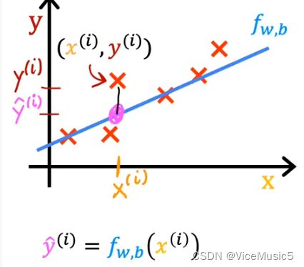
the cost function is written as "J" like J(w,b)

parameters: in this case , w and b are parameters. this term isn`t stand for 'x' that is a part of dataset. we need to confirm a fit model, so the twins are parameter.

ok,there are all notions.Before reading next,I wish you learn or konw what is detivative and slope

The most importent is that the size of J reflects the fitting degree.

How to start a regression in linear ?

(We make a contract : in this article , 'regression' is 'linear regression' without other notice.)

Our goal is find a good model to predict a new input 'x' that computer never sees.A exact and correct linear function is primary.So if we can find suitable a parameter array ’w，b‘ to reduce the sum of the square of error（yi’-yi is a error in one point xi） to minimize even zore。Finally,get the greatest regression model.

If you will understand quickly because you have learned the “最小二乘法”（’二乘‘ means the operation of square），yep .But do you know why we can use it？ it is reasonable and logical?

I can get your confusion.See this viable illusion:

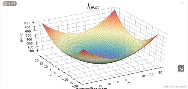
 this is a 3d graph, x-aixs is the value of 'w',y-aixs is the value of 'b', and Z-axis is the value of J with the definitve value of w and b.

We can see the minimize point in blue area(the blackest blue point). In this point , w is xxxx,b is xxxx.......the J is min value in result. In this stiuation,our model fx=wx+b will become the most reasonable fit function in linear model.

Ok,our new goal is defined:Finding w and b to make J smaller.

However,how can we find it?

guess......nonononono

For some another reason(maybe I will tell you my experiment behind),I have learned the "data analyze". For this question ,we can solve by iteration（I do not know whether this expression is right）

For every parameters (such as w),we can iterate it like this:    

( is called 'learning rate',regarded as the size of  iteration step)

repeat this iteration until we can settle at or nccurear a minimize.

A detail that you should pay more attention to: If you have two or more parameters,the upgrade should simultaneously occur! In some algorithms , unsimultaneous upgrade will generate better or lower affect.But you must stick to this, for a stable result.

Well,we saw the 3D-graph minutes ago.Now ,we get a knife and silce a dimension along with x or y-axis:

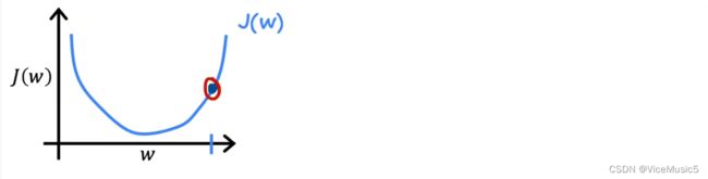
 we need't care another parameter temporarily.Just in it,we can see a point with the smallest J.

Thinking forward,there must exists a array of parameters making J near or reach the minimize If any dimension can find the min point like this.

Now ,let us pay attention to this dimension.Why this iterate function is useful?

Such as this Image,we have a point firstly(we can guess a random value , commonly 0).In the image, we mark it as a red loop.

here,is partial derivative of w.In this dimension,It is the slope of w in this point.(Apparent ,it's positive number),and the a is positive too.

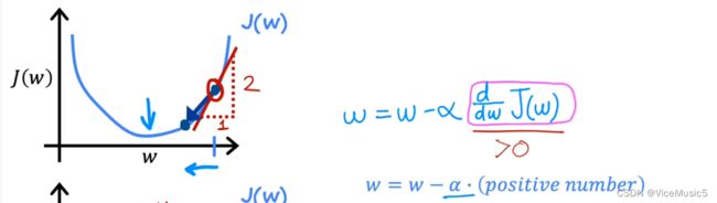
 so ,if we control the size of learning rate, we can make w smaller by reducing a positive number .Until 'w' settle at the target point.

For other parameters, do it.

Now fetch our view back to muti-dimension

 When we complete a upgrade of parameter simultaneously, or finish a iteration of parameters.The point we initied will make a step to lower height,and the value of cost function will smaller than before. This kind of operation is named as 'gradient descent'(梯度下降)

Finally , we can get a suitable array of parameter with one of minimums.In this point , our J can't become smaller near the point(SomeTimes ,you can jump out this 'gap' to find a smaller minimum by use a bigger learning rate,...but it's so dangerous!)

How to judge whether abort the repeative operation of gradient descend?

In the course 'data analyze', the gradience is aborted Until the change was enough little to ignore the increment(增量) in computer counting.Except from this little increment, we can approximately consider it as a suitable minimum.

In the engine aspect，we will say ‘converge’

(why I tell you 'one of'? because if you test another iteratie sequence or different gradient descend direction,you can arrive to a new minimun point and a new cost-value-J)

Are you understand? let us testing!

Use gradient descend to regress

To simplify the process,we only provide two dataMap:(1,2),(2,4)

Define a Linear Function model：

Set original parameters value : w=1 b=1

Spwarl the cos function:

gradient descend algorithms:(repeat until converge):

                                 

finally ,we can have a array [w=2.b=1]

So,we can confirm a correct model

ps:about learning rate

you know, Learning Rate is able to control the step of gradient descend. Definitily,it is limited between 0 to 1.

If it is too small ,like 0.001, the speed of descend will be slow.On the contrary,Too big rate will render 'disverge'