基于时空RBF神经网络的混沌时间序列预测（Matlab代码实现）

 欢迎来到本博客❤️❤️

博主优势：博客内容尽量做到思维缜密，逻辑清晰，为了方便读者。

⛳️座右铭：行百里者，半于九十。

本文目录如下：

目录

1 概述

2 运行结果

3 参考文献

4 Matlab代码实现

---

1 概述

文献来源：

 由于动态性质，混沌时间序列很难预测。在传统的信号处理方法中，信号仅在时域或空间域中处理。信号的时空分析通过利用来自时间和空间域的信息，提供了比传统的一维方法更多的优势。在此，我们提出了一种RBF神经网络的时空扩展，用于预测混沌时间序列。该算法利用时空正交性的概念，分别处理混沌级数的时间动力学和空间非线性（复杂度）。探索了所提出的RBF架构，用于麦基-格拉斯时间序列的预测，并将结果与标准RBF进行了对比。结果表明，时空RBF的性能优于标准RBFNN，可显著降低估计误差。

原文摘要：

Abstract:

Due to the dynamic nature, chaotic time series are difficult predict. In conventional signal processing approaches signals are treated either in time or in space domain only. Spatio-temporal analysis of signal provides more advantages over conventional uni-dimensional approaches by harnessing the information from both the temporal and spatial domains. Herein, we propose an spatio-temporal extension of RBF neural networks for the prediction of chaotic time series. The proposed algorithm utilizes the concept of time-space orthogonality and separately deals with the temporal dynamics and spatial non-linearity(complexity) of the chaotic series. The proposed RBF architecture is explored for the prediction of Mackey-Glass time series and results are compared with the standard RBF. The spatio-temporal RBF is shown to out perform the standard RBFNN by achieving significantly reduced estimation error.

2 运行结果

 

 

 

部分代码：

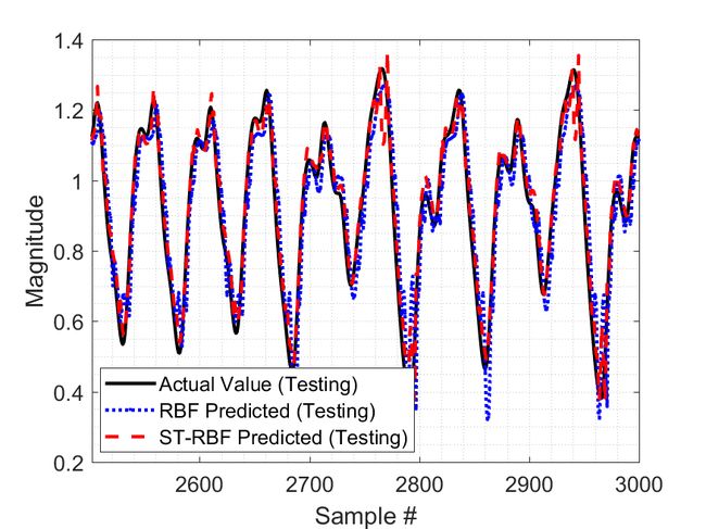
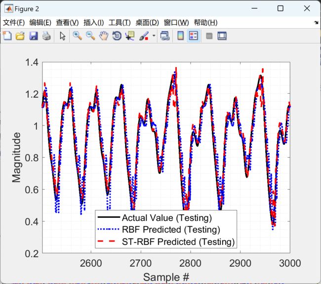
% Input and output signals (test phase)
figure
plot(ST_RBF.indts,ST_RBF.f_test,'k','linewidth',ST_RBF.lw);
hold on;
plot(RBF.indts,RBF.y_test,'.:b','linewidth',RBF.lw);
plot(ST_RBF.indts,ST_RBF.y_test,'--r','linewidth',ST_RBF.lw);
xlim([ST_RBF.start_of_series_ts+ST_RBF.time_steps ST_RBF.end_of_series_ts]);
h=legend('Actual Value (Testing)','RBF Predicted (Testing)','ST-RBF Predicted (Testing)','Location','Best');
grid minor
xlabel('Sample #','FontSize',ST_RBF.fsize);
ylabel('Magnitude','FontSize',ST_RBF.fsize);
set(h,'FontSize',12)
set(gca,'FontSize',13)
saveas(gcf,strcat('Time_SeriesTesting.png'),'png')

% Objective function (MSE) (training phase)
figure
plot(RBF.start_of_series_tr:RBF.end_of_series_tr-1,10*log10(RBF.I(1:RBF.end_of_series_tr-RBF.start_of_series_tr)),'+-b','linewidth',RBF.lw)
hold on
plot(ST_RBF.start_of_series_tr:ST_RBF.end_of_series_tr-1,10*log10(ST_RBF.I(1:ST_RBF.end_of_series_tr-ST_RBF.start_of_series_tr)),'+-r','linewidth',ST_RBF.lw)
h=legend('RBF (Training)','ST-RBF (Training)','Location','North');
grid minor
xlabel('Sample #','FontSize',ST_RBF.fsize);
ylabel('MSE (dB)','FontSize',ST_RBF.fsize);
set(h,'FontSize',12)
set(gca,'FontSize',13)
saveas(gcf,strcat('Time_SeriesTrainingMSE.png'),'png')

% Objective function (MSE) (test phase)
figure
plot(RBF.start_of_series_ts+RBF.time_steps:RBF.end_of_series_ts,10*log10(RBF.I(RBF.end_of_series_tr-RBF.start_of_series_tr+1:end)),'.:b','linewidth',RBF.lw+1)
hold on
plot(ST_RBF.start_of_series_ts+ST_RBF.time_steps:ST_RBF.end_of_series_ts,10*log10(ST_RBF.I(ST_RBF.end_of_series_tr-ST_RBF.start_of_series_tr+1:end)),'.:r','linewidth',ST_RBF.lw+1)
h=legend('RBF (Testing)','ST-RBF (Testing)','Location','South');
grid minor
xlabel('Sample #','FontSize',ST_RBF.fsize);
ylabel('MSE (dB)','FontSize',ST_RBF.fsize);
set(h,'FontSize',12)
set(gca,'FontSize',13)
saveas(gcf,strcat('Time_SeriesTestingMSE.png'),'png')

3 参考文献

部分理论来源于网络，如有侵权请联系删除。

Khan, Shujaat, et al. “A Fractional Gradient Descent-Based RBF Neural Network.” Circuits, Systems, and Signal Processing, vol. 37, no. 12, Springer Nature America, Inc, May 2018, pp. 5311–32, doi:10.1007/s00034-018-0835-3.

Khan, Shujaat, et al. “A Novel Adaptive Kernel for the RBF Neural Networks.” Circuits, Systems, and Signal Processing, vol. 36, no. 4, Springer Nature, July 2016, pp. 1639–53, doi:10.1007/s00034-016-0375-7.

4 Matlab代码实现