机器学习的分类模型评价方法

分类模型评价方法

评估分类器（分类模型）相对于评估回归器通常要复杂，本篇以MNIST数据集的手写数字识别分类为例，记录常用的分类器评估方法。

• 交叉验证：Cross-Validation

  1. 留一交叉验证：（Leave-One-Out Cross Validation记为LOO-CV）在数据缺乏的情况下使用，如果设原始数据有N个样本，那么LOO-CV就是N-CV，即每个样本单独作为验证集，其余的N-1个样本作为训练集，故LOO-CV会得到N个模型，用这N个模型最终的验证集的分类准确率的平均数作为此下LOO-CV分类器的性能指标。

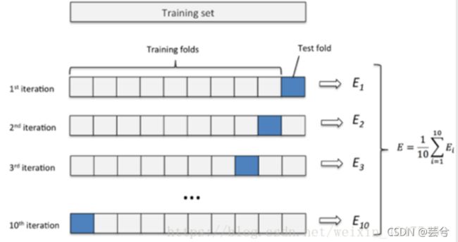
  2. k折交叉验证：将原始数据分成K组（一般是均分），将每个子集数据分别做一次验证集，其余的K-1组子集数据作为训练集，这样会得到K个模型，用这K个模型最终的验证集的分类准确率的平均数作为此K-CV下分类器的性能指标。K一般大于等于2，实际操作时一般从3开始取，只有在原始数据集合数据量小的时候才会尝试取2。

#K折交叉验证
from sklearn.model_selection import cross_val_score
scores=cross_val_score(log_reg, X_pca_3, y, cv=5, scoring='accuracy')
print(scores)  
print("5折交叉验证平均准确率：",np.mean(scores))

交叉验证的局限在于面对样本分布极不均匀的情况下，例如分类正例反例时，样本中正例数目极多，那么分类正例的成功概率自然会很高，如此得到交叉验证的高准确性可信度较低。

混淆矩阵：Confusion Matrix

考虑最简单的二分类情况，分类出错的可能有FP（假正例，原本是反例，误分类为正例），FN（假反例，原本是正例，误分类为反例）。

![在这里插入图片描述](https://img-blog.csdnimg.cn/6d14071004264f7d8bd1656c09977a39.png?x-oss-process=image/watermark,type_ZHJvaWRzYW5zZmFsbGJhY2s,shadow_50,text_Q1NETiBA6Iq45YWu,size_20,color_FFFFFF,t_70,g_se,x_16

from sklearn.metrics import confusion_matrix
def plot_confusion_matrix(clf,name):
    y_pre=clf.predict(X_test)
    confusion=confusion_matrix(y_test,y_pre)
    plt.figure()
    plt.imshow(confusion, cmap=plt.cm.Blues)
    classes = list(set(y_test))
    classes.sort()
    indices = range(len(confusion))
    iters = np.reshape([[[i,j] for j in indices] for i in indices],(confusion.size,2))
    for i, j in iters:
        plt.text(j, i, confusion[i, j])   #显示对应的数字
    plt.title("Confusion matrix of %s "%name,fontsize=12)
    plt.xticks(indices, classes)
    plt.yticks(indices, classes)
    # plt.ylim(len(confusion)-0.5,-0.5)
    plt.xlabel('prediction',fontsize=18)
    plt.ylabel('reality',fontsize=18)
    
plot_confusion_matrix(log_reg,'LogistRegression')`

混淆矩阵沿着主对角线的分布集中度越高，代表模型的分类精度越高。

• 精确率&召回率（查准率&查全率）：Precision and Recall

$$P=TP/(TP+FP)$$
精确率针对预测结果而言，又称查准率，即预测结果中预测正确的正样本所占总预测次数的比率，该值越大证明预测结果的准确率越高
$$R=TP/(TP+FN)$$

召回率针对原有样本而言，又成查全率，即预测模型预测正确的正样本占总的真实样本的比率，该值越大证明预测结果中预测到的正例数相对于样本中实际的正例数越全。所谓召回，可理解为真实的正例数在预测中再次预测出，即被召回。

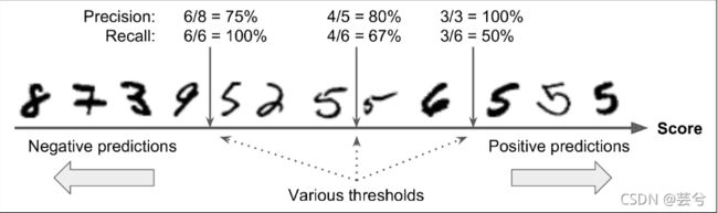
• 精确率/召回率权衡 ：Precision/Recall Tradeoff
  精确率与召回率通常无法同时取得比较理想的结果，考虑实际中模型5分类器预测的过程，模型通过训练最终得到一个判断的阈值threshold，高于threshold判断为5，反之为非5，显而易见的时，当高阈值的情况下精确性更高，而低阈值的情况下召回率更高，即分类模型可囊括的真实正实例5的数目越多。
  

高精确率和高召回率的取舍通常取决于我们需要解决的实际问题，例如我们要训练一个视频分类器，以避免将不好的内容推送给用户时，假如这里的5代表健康的视频，那么我们倾向于模型具有更高的准确性，以保证推送给用户的视频尽可能的健康，尽管这样可能会导致召回率的下降，即将一些原本健康的视频分到问题视频的类别中；在另一种情况下，考虑机场视频监控中可疑扒手识别模型中，假如这里的5代表偷窃行为，那么我们更倾向于模型能够具有更高的召回率，以尽可能地不放过任何一个扒手，尽管这样做可能会导致模型准确性下降，以至于错误警报增多。
准确率与召回率的权衡也可能通过绘制以准确率和召回率为坐标轴的图像曲线来看，通常称为PR曲线：

通过该图，结合自己的实际情况，可以在确保精确率或者召回率一方达到要求的同时，仅可能选择另一参数更高的阈值，来得到符合期望的模型效果。

此外，当模型的准确率和召回率相近时，可以使用准确率和召回率的调和平均数，通常称为F1得分，来评价模型分数
$$F_1=\frac{2}{\frac{1}{\text{ precision }}+\frac{1}{\text{ recall }}}=2\times \frac{\text{ precision }\times \text{ recall }}{\text{ precision }+\text{ recall }}=\frac{TP}{TP+\frac{FN+FP}{2}}$$

• 受试者工作特征曲线：receiver operating characteristic (ROC) curve

得此名的原因在于曲线上各点反映着相同的感受性，它们都是对同一信号刺激的反应，只不过是在几种不同的判定标准下所得的结果而已。
它与精确率/召回率曲线非常相似，但 ROC 曲线不是绘制精确率与召回率的关系图，而是绘制真阳性率（召回的另一个名称）与假阳性率的关系图。所谓真阳性率即为召回率，而假阳性率(false positive rate)，即真实为阴性的被误认为是阳性的样本占原有样本的比率，它等价于1-真阴性率，真阴性率即真实为阴性且预测为阴性所在预测样本中的比率，真阴性率可以称为以阴性为主的准确率。
$$TPR=TP/(TP+FN)$$
$$FPR=FP/(FP+TN)=1-TNR$$
$$TNR=TN/(TN+FP)$$

FPR和TPR曲线同样具有类似准确率和召回率那样的权衡，上图虚线代表随机分类器的结果，一个好的分类器会尽可能的远离该虚线。
一种比较分类器好坏的方法是比较ROC曲线下方的面积（Area Under the Curve），面积接近为1的分类器是最为理想的。
ROC曲线和PR曲线是十分类似的，经验法则告诉我们，当样本中阳性例数目较少，或者我们更加关心假阳性（假阳性为小概率）时，选择PR曲线，反之选择ROC曲线。

# -*- coding: utf-8 -*-
"""
Created on Tue Oct  5 19:17:58 2021

@author: Flower unbeaten
"""
import sys
assert sys.version_info >= (3, 5)

#Scikit-Learn ≥0.20 is required
import sklearn
assert sklearn.__version__ >= "0.20"
import numpy as np
import os
np.random.seed(42)

#plot pretty figures
#引入画图库，提前设置好绘图坐标标签大小等参数
import matplotlib as mpl
import matplotlib.pyplot as plt
plt.rcParams['font.family'] = 'SimHei'
plt.rcParams['axes.unicode_minus'] = False#绘图准备
mpl.rc('axes',labelsize=14)
mpl.rc('xtick',labelsize=12)
mpl.rc('ytick',labelsize=12)

#figures save path
#静态变量统一使用大写字母+下划线分割，"."代表当前目录，os.makedirs(“保存路径”,exist_ok)
#exist_ok为true时当文件夹已经存在时不会提示异常，为false时则会
PROJECT_ROOT_DIR = "."
CHAPTER_ID = "classification"
IMAGES_PATH = os.path.join(PROJECT_ROOT_DIR,"images",CHAPTER_ID)
os.makedirs(IMAGES_PATH,exist_ok = True)

#save figure function
def save_fig(fig_id, tight_layout=True, fig_extension="png",resolution=300):
    path = os.path.join(IMAGES_PATH, fig_id + "." + fig_extension)
    print("Saving figure", fig_id)
    if tight_layout:
        plt.tight_layout()
        plt.savefig(path, format=fig_extension, dpi=resolution)

#import MNIST dataset
from sklearn.datasets import fetch_openml
mnist = fetch_openml('mnist_784',version=1)
mnist.keys()

#overview the data
X, y = mnist["data"] , mnist["target"]
print("X大小为", X.shape)
print("y大小为", y.shape)

#类型转化
#数据类型原本为DataFrame，表头索引对数据进行说明，这里我们仅关注数据本身，
#使用DataFrame、Series的values属性转为array类型
X = X.values
y = y.values

#取一个图片看看
some_digit = X[0]
some_digit_image = some_digit.reshape(28,28)
#cmap指代colormap，指定为二值图
plt.imshow(some_digit_image, cmap=mpl.cm.binary)
plt.axis("off")

#显示第一个数字图片，查看对应的target标签
save_fig("some_digit_plot")
print("对应的标签为", y[0])

y = y.astype(np.uint8)

def plot_digit(data):
    image = data.reshape(28,28)
    plt.imshow(image,cmap = mpl.cm.binary,interpolation="nearest")
    plt.axis("off")
    
#绘制一片数字
def plot_digits(instances,images_per_row=10,**options):
    size = 28
    images_per_row = min(len(instances),images_per_row)
    images = [np.array(instance).reshape(size,size) for instance in instances]
    n_rows = (len(instances)) // images_per_row + 1
    row_images = []
    n_empty = n_rows*images_per_row - len(instances)
    images.append(np.zeros((size,size*n_empty)))
    for row in range(n_rows):
        rimages = images[row*images_per_row : (row+1)*images_per_row]
        row_images.append(np.concatenate(rimages,axis = 1))
    image = np.concatenate(row_images,axis=0)
    plt.imshow(image , cmap = mpl.cm.binary,**options)
    plt.axis("off")
    
plt.figure(figsize=(9,9))
example_images = X[:100]
plot_digits(example_images,images_per_row=10)
save_fig("more_digits_plot")
plt.show()

#数据集划分
#MNIST数据集的训练集已经被随机打乱并划分好，前60000个为训练集，其余为测试集
X_train, X_test, y_train, y_test = X[:60000], X[60000:], y[:60000], y[60000:]

#训练一个判断数字是否为5的二分类器
#这里的标签为布尔型，5为true，非5为false
y_train_5 =( y_train == 5)
y_test_5 = (y_test == 5)
y_5 = (y == 5)
#引入SGD分类器模型
from sklearn.linear_model import SGDClassifier
#tol为停止标准，即精度小于tol时停止，max_iter,最大迭代次数，iteration，迭代
sgd_clf = SGDClassifier(max_iter=1000, tol=1e-3, random_state=42)
#使用训练集训练模型
#通常我们想要记录训练花费时间，引入time包，使用time.time()方法记录
import time
tic = time.time()
sgd_clf.fit(X_train, y_train_5)
toc = time.time()
print("SGDClassifier cost",(toc-tic),"s" )

#调用我们训练好的模型来识别之前的some_digit，使用sgd_clf.predict
print("训练完成的模型判断some_digit是否为5的结论是",sgd_clf.predict([some_digit]))

## 分类模型评价
#K折交叉验证
from sklearn.model_selection import cross_val_score
scores=cross_val_score(sgd_clf, X, y_5, cv=3, scoring='accuracy')
print("每折准确率为：", scores)
print("3折交叉验证平均准确率：",np.mean(scores))

#也可以不用模型自带的cross_val_score，自己实现交叉验证的过程
#引入克隆器，用于克隆已经使用某折数据训练过的模型
from sklearn.model_selection import StratifiedKFold
from sklearn.base import clone
#划分3折,创建一个三折数据划分器
skfolds = StratifiedKFold(n_splits =3)
#每一折单独划分训练集与测试集，每次训练得到的模型被克隆得到保存，后边的数据折在前边训练得到的模型基础上继续训练
for train_index , test_index in skfolds.split(X_train, y_train_5):
    #k折划分留一折作为测试集，其余为训练集
    clone_clf = clone(sgd_clf)
    X_train_folds = X_train[train_index]
    y_train_folds = y_train_5[train_index]
    X_test_fold = X_train[test_index]
    y_test_fold = y_train_5[test_index]
    
    #使用训练集折训练模型，对测试集进行预测，将结果与实际测试集targe比对，得到正确数目
    clone_clf.fit(X_train_folds, y_train_folds)
    y_pred = clone_clf.predict(X_test_fold)
    n_correct = sum(y_pred == y_test_fold)
    #计算准确率
    print(n_correct / len(y_pred))
    
#混淆矩阵
from sklearn.metrics import confusion_matrix
#confusion matrix function
def plot_confusion_matrix(clf,name,X_test,y_test):
    y_pre=clf.predict(X_test)
    confusion=confusion_matrix(y_test,y_pre)
    plt.figure()
    plt.imshow(confusion, cmap=plt.cm.Oranges)
    classes = list(set(y_test))
    classes.sort()
    indices = range(len(confusion))
    iters = np.reshape([[[i,j] for j in indices] for i in indices],(confusion.size,2))
    for i, j in iters:
        plt.text(j, i, confusion[i, j])   #显示对应的数字
    plt.title("Confusion matrix of %s "%name,fontsize=12)
    plt.xticks(indices, classes)
    plt.yticks(indices, classes)
    # plt.ylim(len(confusion)-0.5,-0.5)
    plt.xlabel('prediction',fontsize=18)
    plt.ylabel('reality',fontsize=18)
    
plot_confusion_matrix(sgd_clf,'SGDClassifier',X_test,y_test_5)
save_fig("SGDClassifier confusion matrix plot")

# PR(准确率/召回率曲线)
#导入PR计算函数，PR曲线函数
from sklearn.metrics import precision_recall_curve
from sklearn.metrics import precision_score, recall_score
from sklearn.metrics import f1_score
#计算训练集的PR，F1score，这里也可以自己根据公式来计算
y_train_pred = sgd_clf.predict(X_train)
sgd_precision = precision_score(y_train_5, y_train_pred)
sgd_recall = recall_score(y_train_5, y_train_pred)
sgd_f1score = f1_score(y_train_5, y_train_pred)
print("P:",sgd_precision)
print("R:",sgd_recall)
print("F1:",sgd_f1score)

#使用cross_val_predict决策函数返回实例的预测分数，而非预测类别
#该函数也可在生成混淆矩阵时使用，那个时候是预测类别
from sklearn.model_selection import cross_val_predict
y_scores = cross_val_predict(sgd_clf, X_train, y_train_5, cv=3,
                             method="decision_function")
precisions, recalls, thresholds = precision_recall_curve(y_train_5, y_scores)
#定义PR曲线绘制函数
def plot_precision_vs_recall(precisions, recalls):
    plt.plot(recalls, precisions, "b-", linewidth=2)
    plt.xlabel("Recall", fontsize=16)
    plt.ylabel("Precision", fontsize=16)
    plt.axis([0, 1, 0, 1])
    plt.grid(True)
plt.figure(figsize=(8, 6))
plot_precision_vs_recall(precisions, recalls)
save_fig("precision_vs_recall_plot")
plt.show()

#ROC curves 受试者工作曲线
from sklearn.metrics import roc_curve

fpr, tpr, thresholds = roc_curve(y_train_5, y_scores)

def plot_roc_curve(fpr, tpr, label=None):
    plt.plot(fpr, tpr, linewidth=2, label=label)
    plt.plot([0, 1], [0, 1], 'k--') # dashed diagonal
    plt.axis([0, 1, 0, 1])
    plt.xlabel('False Positive Rate (Fall-Out)', fontsize=16)
    plt.ylabel('True Positive Rate (Recall)', fontsize=16)
    plt.grid(True)                

plt.figure(figsize=(8, 6))
plot_roc_curve(fpr, tpr)
save_fig("roc_curve_plot")
plt.show()

#使用auc（roc曲线下方面积）打分模型
from sklearn.metrics import roc_auc_score

print("auc得分：", roc_auc_score(y_train_5, y_scores))