High Dynamic Range Imaging(高动态范围图片HDR合成)

High Dynamic Range Imaging

高动态范围(HDR)图像合成 OUC_Shizue

What is High Dynamic Range（HDR）Imaging?

​ Most digital cameras and displays capture or display color images as 24-bits matrices. There are 8-bits per color channel and the pixel values are therefore in the range 0–255 for each channel. In other words, a regular camera or a display has a limited dynamic range.

​ However, the world around us has a very large dynamic range. It can get pitch black inside a garage when the lights are turned off and it can get really bright if you are looking directly at the Sun. Even without considering those extremes, in everyday situations, 8-bits are barely enough to capture the scene. So, the camera tries to estimate the lighting and automatically sets the exposure so that the most interesting aspect of the image has good dynamic range, and the parts that are too dark and too bright are clipped off to 0 and 255 respectively.

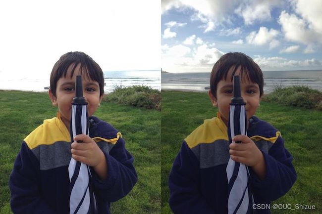
​ In the Figure below, the image on the left is a normally exposed image. Notice the sky in the background is completely washed out because the camera decided to use a setting where the subject (a boy) is properly photographed, but the bright sky is washed out. The image on the right is an HDR image produced by the iPhone.

​ How does an iPhone capture an HDR image? It actually takes 3 images at three different exposures. The images are taken in quick succession so there is almost no movement between the three shots. The three images are then combined to produce the HDR image. We will see the details in the next section.

The process of combining different images of the same scene acquired under different exposure settings is called High Dynamic Range (HDR) imaging.

​ To summarize，High dynamic range (HDR，高动态范围)have much larger dynamic range than traditional images’ 256 brightness levels. In addition, they correspond linearly to physical irradiance values of the scene. Hence, they have many applications in graphics and vision. In this project, you are expected to finish the following tasks to assemble an HDR image.

Step 1:Capture multiple images with different exposures

1、论文

​ Taking images. Taking a series of photographs for a scene under different exposures. As discussed in the class, changing shutter speed is probably the best way to change exposure for this application. For that, you need a digital camera that allows you to set exposures. (Note that not every camera allows a user to manually set exposures.) You can use your own camera on your cellphone.

​ One thing to note is that you should avoid moving your camera during this process so that all pictures are well registered. Some digital cameras have their own programs which allow users to remotely control the shutters via their USB cables. Using such programs prevent you from shaking the camera while pressing the shutter. You are welcome to write down your findings for that matter in your report.

2、总结

• 用不同的曝光时间拍摄多张照片，拍摄过程中要保持相对静止，防止多张图片错位。建议使用三脚架+usb控制拍摄，最大幅度减小抖动。
• 同时拍摄的每张图片要记录其对应的曝光时间，便于后续求解。

3、拍摄结束后从文件夹将图片和曝光时间导入python代码中

import os
import cv2
import matplotlib.pyplot as plt
import numpy as np
#% matplotlib inline
#% config InlineBackend.figure_format = 'svg'

# 从文件夹中读取图片路径
def getPath(filePath):
    paths = []
    for root, dirs, files in os.walk(filePath):
        if root != filePath:
            break
        for file in files:
            path = os.path.join(root, file)
            paths.append(path)
            #print(path)
    for i in paths:
        if 'txt' in i:
            index = paths.index(i)
    paths.remove(paths[index])
    #print(paths)
    return paths


# 根据路径列表使用cv2将图片读成np.array格式
def getImages(filePath):
    paths = getPath(filePath)
    img = [cv2.imread(x) for x in paths]
    return img


# 从txt文件中读出曝光时间，返回列表
def getTimes(path):
    times = []
    with open(path, 'r') as fp:
        line = [x.strip() for x in fp]
    for i in line:
        times.append(eval(i[6:]))
    times = np.array(times).astype(np.float32)
    return times

这里文件夹内容为/dir/[1.jpg,2.jpg,expoture.txt],txt文件内为[img01:10,img02:4]依次类推。

调用方式举例:

images = getImages('./exposures/')
times = getTimes("./exposures/shutter.txt")

# plt查看图片是否读入成功
plt.imshow(images[0])

Step 2:Align Images

1、论文

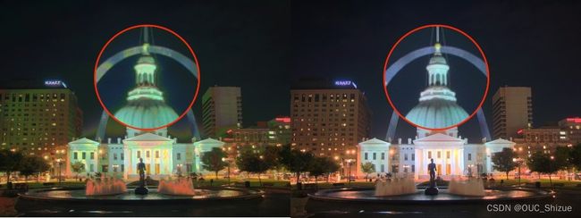
​ Misalignment of images used in composing the HDR image can result in severe artifacts. In the Figure below, the image on the left is an HDR image composed using unaligned images and the image on the right is one using aligned images. By zooming into a part of the image, shown using red circles, we see severe ghosting artifacts in the left image.

​ Naturally, while taking the pictures for creating an HDR image, professional photographer mount the camera on a tripod. They also use a feature called mirror lockup to reduce additional vibrations. Even then, the images may not be perfectly aligned because there is no way to guarantee a vibration-free environment. The problem of alignment gets a lot worse when images are taken using a handheld camera or a phone.

​ Fortunately, OpenCV provides an easy way to align these images using AlignMTB. This algorithm converts all the images to median threshold bitmaps (MTB). An MTB for an image is calculated by assigning the value 1 to pixels brighter than median luminance and 0 otherwise. An MTB is invariant to the exposure time. Therefore, the MTBs can be aligned without requiring us to specify the exposure time.

​ MTB based alignment is performed using the following lines of code.

2、总结

多张图片合成一张HDR过程中，由于像素点偏差可能出现合成后无法对齐，因此可以使用OpenCV内置对齐函数对多张图片先对齐，再进行合成。

代码如下:

alignMTB = cv2.createAlignMTB()
alignMTB.process(images, images)

Step 3:Recover the Camera Response Function

1、论文

​ Write a program to assemble an HDR image. Write a program to take these captured images as inputs and output an HDR image as well as the response curve of the camera. You will use the Debevec's method. Please refer to Debevec’s SIGGRAPH 1997 paper below. The most difficult part probably is to solve the over-determined linear system.

​ Paul E. Debevec, Jitendra Malik, Recovering High Dynamic Range Radiance Maps from Photographs, SIGGRAPH 1997.

​ The response of a typical camera is not linear to scene brightness. What does that mean? Suppose, two objects are photographed by a camera and one of them is twice as bright as the other in the real world. When you measure the pixel intensities of the two objects in the photograph, the pixel values of the brighter object will not be twice that of the darker object! Without estimating the Camera Response Function (CRF), we will not be able to merge the images into one HDR image.

What does it mean to merge multiple exposure images into an HDR image?

​ Consider just ONE pixel at some location (x,y) of the images. If the CRF was linear, the pixel value would be directly proportional to the exposure time unless the pixel is too dark ( i.e. nearly 0 ) or too bright ( i.e. nearly 255) in a particular image. We can filter out these bad pixels ( too dark or too bright ), and estimate the brightness at a pixel by dividing the pixel value by the exposure time and then averaging this brightness value across all images where the pixel is not bad ( too dark or too bright ). We can do this for all pixels and obtain a single image where all pixels are obtained by averaging “good” pixels.

​ But the CRF is not linear and we need to make the image intensities linear before we can merge/average them by first estimating the CRF.

​ The good news is that the CRF can be estimated from the images if we know the exposure times for each image. Like many problems in computer vision, the problem of finding the CRF is set up as an optimization problem where the goal is to minimize an objective function consisting of a data term and a smoothness term. These problems usually reduce to a linear least squares problem which are solved using Singular Value Decomposition (SVD) that is part of all linear algebra packages. The details of the CRF recovery algorithm are in the paper titled Recovering High Dynamic Range Radiance Maps from Photographs.

2、总结

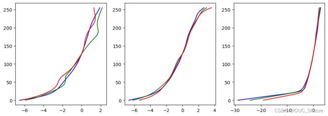
这一步为核心，即求解相机响应曲线CRF，底层原理为求解一个方程，由于只需要0~255个参数，因此可以直接从我们的图片中选择大于等于255组数据代入即可求出CRF。对应方程如图:

Debevec教授在论文中给出了详细求解步骤以及对应简洁的MATLAB代码，可供参考。

3、代码实现

（1）拆分通道以及SVD求解函数

# 将图片拆分为三通道
def split(images):
    i_b, i_g, i_r = [], [], []
    for i in images:
        b, g, r = cv2.split(i)
        i_b.append(b)
        i_g.append(g)
        i_r.append(r)
    return i_b, i_g, i_r


# 设置权重
def wei(z, zmin=0, zmax=255):
    zmid = (zmin + zmax) / 2
    return z - zmin if z <= zmid else zmax - z


# 响应曲线求解
def gsolve(Z, B, l, w):
    n = 256
    A = np.zeros(shape=(np.size(Z, 0) * np.size(Z, 1) + n + 1, n + np.size(Z, 0)), dtype=np.float32)
    b = np.zeros(shape=(np.size(A, 0), 1), dtype=np.float32)

    # Include the data−fitting equations
    k = 0
    for i in range(np.size(Z, 0)):
        for j in range(np.size(Z, 1)):
            z = int(Z[i][j])
            wij = w[z]
            A[k][z] = wij
            A[k][n + i] = -wij
            b[k] = wij * B[j]
            k += 1
    # Fix the curve by setting its middle value to 0
    A[k][128] = 1
    k += 1
    # 平滑处理
    for i in range(n - 1):
        A[k][i] = l * w[i + 1]
        A[k][i + 1] = -2 * l * w[i + 1]
        A[k][i + 2] = l * w[i + 1]
        k += 1
    # 使用SVD求解
    x = np.linalg.lstsq(A, b, rcond=None)[0]
    g = x[:256]
    lE = x[256:]

    return g, lE

（2）随机取点代入求解

import random


# 第一步：随机取N个点
def hdr_debvec(images, times, l, sample_num):
    global w
    B = np.log2(times)
    w = [wei(z) for z in range(256)]
    samples = [(random.randint(0, images[0].shape[0] - 1), random.randint(0, images[0].shape[1] - 1)) for i in
               range(sample_num)]
    Z = []
    for img in images:
        Z += [[img[r[0]][r[1]] for r in samples]]
    Z = np.array(Z).T
    return gsolve(Z, B, l, w)


# 调用通道拆分函数，将各个通道对应数组、曝光时间送入gslove求解g、lE
def getCRF(images, times, l=10, sam_num=70):
    _b, _g, _r = split(images)
    image_gb, lEb = hdr_debvec(_b, times, l, sam_num)
    image_gg, lEg = hdr_debvec(_g, times, l, sam_num)
    image_gr, lEr = hdr_debvec(_r, times, l, sam_num)
    # 返回三个通道对应g、lE
    return [image_gb, image_gg, image_gr]

(3)可视化

# 调用函数得到三通道的CRF
plt.figure(figsize=(12, 4))

# 由于我一次做了三组合成，此处n为第几组数据
def rgbShow(images, times, n, l=50):
    crf = getCRF(images, times, l)
    plt.subplot(1, 3, n)
    plt.plot(crf[0], range(256), 'b')
    plt.plot(crf[1], range(256), 'g')
    plt.plot(crf[2], range(256), 'r')


rgbShow(images1, times1, 1, l=50)
rgbShow(images2, times2, 2, l=50)
rgbShow(images3, times3, 3, l=50)

Step 3:Merge Images

总结

这一步很简单，即使用上述CRF将多张图片合成一张.hrd图片，实现如下：

# 用opencv函数合成HDR图片
plt.figure(figsize=(15, 6))


def showimg(images, times, respon, n):
    merge = cv2.createMergeDebevec()
    hdrDeb = merge.process(images, times, respon)
    plt.subplot(1, 3, n)
    plt.imshow(cv2.cvtColor(hdrDeb, cv2.COLOR_BGR2RGB))


showimg(images1, times1, responseDebevec1, 1)
showimg(images2, times2, responseDebevec2, 2)
showimg(images3, times3, responseDebevec3, 3)

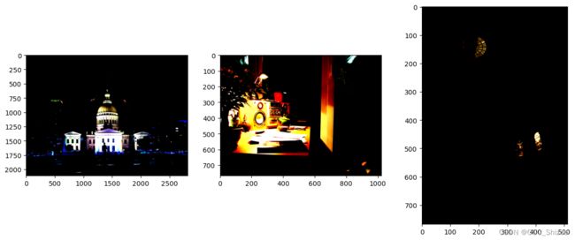
恢复辐照图，代码实现如下:

### TODO: recover the radiance map
def OneMap(images, times, g):
    tizu = np.zeros((images[0].shape[0], images[0].shape[1]))
    sumDown = np.zeros((images[0].shape[0], images[0].shape[1]))
    w = np.array([wei(z) for z in range(256)])
    for k in range(len(times)):
        Zij = images[k]
        Wij = w[Zij]
        tizu += Wij * (g[Zij][:, :, 0] - np.log(times[k]))
        sumDown += Wij
    tizu = tizu / sumDown
    return tizu


def RadianceMap(images, times, crf):
    images_b, images_g, images_r = split(images)
    radiancemap = np.zeros((images[0].shape[0], images[0].shape[1], 3), dtype=np.float32)
    radiancemap[:, :, 0] = OneMap(images_b, times, crf[0])
    radiancemap[:, :, 1] = OneMap(images_g, times, crf[1])
    radiancemap[:, :, 2] = OneMap(images_r, times, crf[2])
    return radiancemap


radiancemap1 = RadianceMap(images1, times1, getCRF(images1, times1, l=50))
radiancemap2 = RadianceMap(images2, times2, getCRF(images2, times2, l=50))
radiancemap3 = RadianceMap(images3, times3, getCRF(images3, times3, l=50))

# plot your radiance map
plt.figure(figsize=(15, 6))
plt.subplot(1, 3, 1)
plt.imshow(radiancemap1)
plt.subplot(1, 3, 2)
plt.imshow(cv2.cvtColor(radiancemap2, cv2.COLOR_BGR2RGB))
plt.subplot(1, 3, 3)
plt.imshow(cv2.cvtColor(radiancemap3, cv2.COLOR_BGR2RGB))

Step 4:Tone Mapping

1、论文

​ Now we have merged our exposure images into one HDR image. Can you guess the minimum and maximum pixel values for this image? The minimum value is obviously 0 for a pitch black condition. What is the theoretical maximum value? Infinite! In practice, the maximum value is different for different situations. If the scene contains a very bright light source, we will see a very large maximum value.

​ Even though we have recovered the relative brightness information using multiple images, we now have the challenge of saving this information as a 24-bit image for display purposes.

The process of converting a High Dynamic Range (HDR) image to an 8-bit per channel image while preserving as much detail as possible is called Tone mapping.

​ There are several tone mapping algorithms. OpenCV implements four of them. The thing to keep in mind is that there is no right way to do tone mapping. Usually, we want to see more detail in the tonemapped image than in any one of the exposure images. Sometimes the goal of tone mapping is to produce realistic images and often times the goal is to produce surreal images. The algorithms implemented in OpenCV tend to produce realistic and therefore less dramatic results.

​ Let’s look at the various options. Some of the common parameters of the different tone mapping algorithms are listed below.

• gamma : This parameter compresses the dynamic range by applying a gamma correction. When gamma is equal to 1, no correction is applied. A gamma of less than 1 darkens the image, while a gamma greater than 1 brightens the image.
• saturation : This parameter is used to increase or decrease the amount of saturation. When saturation is high, the colors are richer and more intense. Saturation value closer to zero, makes the colors fade away to grayscale.
• contrast : Controls the contrast ( i.e. log (maxPixelValue/minPixelValue) ) of the output image.

Let us explore one of the tone mapping algorithms available in OpenCV.

Reinhard Tonemap

createTonemapReinhard
(
float   gamma = 1.0f,
float   intensity = 0.0f,
float   light_adapt = 1.0f,
float   color_adapt = 0.0f
)

​ The parameter intensity should be in the [-8, 8] range. Greater intensity value produces brighter results. light_adapt controls the light adaptation and is in the [0, 1] range. A value of 1 indicates adaptation based only on pixel value and a value of 0 indicates global adaptation. An in-between value can be used for a weighted combination of the two. The parameter color_adapt controls chromatic adaptation and is in the [0, 1] range. The channels are treated independently if the value is set to 1 and the adaptation level is the same for every channel if the value is set to 0. An in-between value can be used for a weighted combination of the two.

For more details, check out this paper.

2、总结

​ 将上述hdr图片做色调映射，转化为目标图片

3、代码实现

import matplotlib.pyplot as plt


### TODO: Call OpenCV's function to tonemap the radiance map you have recovered.
def imgWrite(radianceMap, n):
    tonemap = cv2.createTonemapDrago(0.25, 0.5)
    ldrImg = tonemap.process(radianceMap)
    ldrImg = 3 * ldrImg
    cv2.imwrite("output/ldrDrago" + str(n) + ".jpg", ldrImg * 255)


imgWrite(radiancemap1, 1)
imgWrite(radiancemap2, 2)
imgWrite(radiancemap3, 3)

plt.figure(figsize=(12, 4))


def imgShow(path, n):
    HDRimg = cv2.imread(path)
    plt.subplot(1, 3, n)
    plt.imshow(cv2.cvtColor(HDRimg, cv2.COLOR_BGR2RGB))


imgShow("output/ldrDrago1.jpg", 1)
imgShow("output/ldrDrago2.jpg", 2)
imgShow("output/ldrDrago3.jpg", 3)

References

Book

• High dynamic range imaging: acquisition, display, and image-based lighting
  • Reinhard, Erik, et al. ,2010
  • The bible of the HDR imaging

HDR Image Reconstruction

• Debevec, Paul E., and Jitendra Malik. “Recovering high dynamic range radiance maps from photographs.” Proceedings of the 24th annual conference on Computer graphics and interactive techniques. ACM Press/Addison-Wesley Publishing Co., 1997.
  • The basic but effective method for HDR image reconstruction, this paper motivates many works about HDR imaging
  • Matrix form solution(including least square term and smoothness term)
• Robertson, Mark, Sean Borman, and Robert L. Stevenson. “Dynamic range improvement through multiple exposures.” Image Processing, 1999. ICIP 99. Proceedings. 1999 International Conference on. Vol. 3. IEEE, 1999.
  • Maximum likelihood solution, consider the additive noise and dequantization error as independent Gaussian random variable
  • Iterative method derived from the partial differential equation results
• Mitsunaga, Tomoo, and Shree K. Nayar. “Radiometric self calibration.” Computer Vision and Pattern Recognition, 1999. IEEE Computer Society Conference on… Vol. 1. IEEE, 1999.
  • Use polynomials to model the CRF
  • Iterative method with rough estimation of exposure time ratio
• Lin, Stephen, et al. “Radiometric calibration from a single image.” Computer Vision and Pattern Recognition, 2004. CVPR 2004. Proceedings of the 2004 IEEE Computer Society Conference on. Vol. 2. IEEE, 2004.
  • Single image HDR scheme
  • Based on the edge color distribution

Image Alignment and Registration

• Ward, Greg. “Fast, robust image registration for compositing high dynamic range photographs from hand-held exposures.” Journal of graphics tools 8.2 (2003): 17-30.
  • Median threshold bitmap (MTB) for global alignment
  • Very efficient (due to based on bitwise operation)
• Kang, Sing Bing, et al. “High dynamic range video.” ACM Transactions on Graphics (TOG) 22.3 (2003): 319-325.
  • Both global and local registration
  • A variant of LK optical flow
  • A strategy to obtain HDR video

Alternative to HDR imaging
Exposure Fusion
Two series of paper

• Mertens, Tom, Jan Kautz, and Frank Van Reeth. “Exposure fusion.” Computer Graphics and Applications, 2007. PG’07. 15th Pacific Conference on. IEEE, 2007.
• Mertens, Tom, Jan Kautz, and Frank Van Reeth. “Exposure fusion: A simple and practical alternative to high dynamic range photography.” Computer Graphics Forum. Vol. 28. No. 1. Blackwell Publishing Ltd, 2009.
  ative to HDR imaging
  Exposure Fusion
  Two series of paper
• Mertens, Tom, Jan Kautz, and Frank Van Reeth. “Exposure fusion.” Computer Graphics and Applications, 2007. PG’07. 15th Pacific Conference on. IEEE, 2007.
• Mertens, Tom, Jan Kautz, and Frank Van Reeth. “Exposure fusion: A simple and practical alternative to high dynamic range photography.” Computer Graphics Forum. Vol. 28. No. 1. Blackwell Publishing Ltd, 2009.
  • Scalar-weighted map is first generated based on the quality measurement (contrast, saturation, well-exposedness) of the exposure bracketed image, then the fusion is performed in the multiresolution manner (Each layer of the Laplacian pyramid of resulting image is computed by the pixel-based multiplication if Gaussian pyramids of the weighted map with Laplacian pyramids of the original image)