协同多种SAR数据及多光谱数据的星载激光雷达GEDI森林生物量估测

协同多种SAR数据及多光谱数据的星载激光雷达GEDI森林生物量估测

GEDI生物量估测的现实应用

前段时间，基本梳理了一下ICESat-2与GEDI树高相关研究的一些知识点。近段时间，有看到很多学者做了关于利用GEDI数据进行生物量估测一些文章。结合前段时间利用多源数据与GEDI和ICESat-2反演树高的一些方法。我想着能不能同样利用多源数据来实现从点到面的GEDI生物量估测。实现出一个较为完整的生物量估测流程。无独有偶，NASA官方公布了GEDI对GEE的数据集，这给实现云端多数据协同反演生物量提供了一个很大便利。

多源数据的选择

在反演树高的时候，学者采用了Sentinel-1 SAR双极化数据，以及Sentinel-2多光谱数据，这两个数据的优点在于可以白嫖，Sentinel-1使用C波段（波长为5.6厘米），这意味着它具有穿透云层和雨的能力，能够在各种天气条件下进行观测。Sentinel-1可以以多种观测模式进行数据采集，包括窄波束、宽波束和交叉极化，这使其能够适应不同应用领域的需求。Sentinel-2使用多光谱成像仪（MSI）进行观测，具有多个光谱波段（从可见光到近红外），使其在地表覆盖分类、植被监测、土地利用变化等方面非常有用。同时，具有较短的重访周期，可以在短时间内获取多个地区的数据，使其在监测快速变化的地理现象时非常有用。但是Sentinel-1的C波段可能限制了一些对不同频段数据进行比较分析的应用。日本宇宙航空研究开发机构（JAXA）开发的合成孔径雷达（SAR）卫星PALSAR-2（Phased Array type L-band Synthetic Aperture Radar-2）数据，工作在L波段（波长约为23.5厘米），相较于可见光和红外波段，L波段的微波具有较强的穿透能力，能够穿透云层和雨雪覆盖，以及对地表下的土壤和植被进行探测。
PALSAR-2可以以不同的观测模式进行数据采集，包括极化模式、干涉模式和极化干涉模式。这使得它能够提供不同类型的数据产品，适用于不同的应用领域，如土地利用、森林监测、冰川变化等。PALSAR-2提供了较高的空间分辨率，可达到1米至10米不等，这使其能够提供更精细的地表特征信息。高分辨率的数据对于地表变化监测、地貌分析和目标检测等应用非常有用。PALSAR-2具有较长的重访周期，可以在相同地区进行多次观测，形成长时间序列的数据。这对于研究地表变化、监测自然灾害和评估环境影响非常有益。由于使用微波频段，PALSAR-2具有全天候观测能力，不受天气条件的限制。它可以在夜晚、阴雨天或云层遮挡下获取数据，提供持续观测的能力。
在多源数据协作的时候，学者综上选择了Sentinel-1、Sentinel-2、PALSAR-2、SRTM-DEM以及林分数据（用于掩膜森林区域）等等。

加载数据

1. 加载GEDI数据集

var l4b = ee.Image('LARSE/GEDI/GEDI04_B_002');
var dataset = l4b.select('MU').clip(roi);//选取平均生物量字段
//投影                  
var dataset = dataset.reproject({crs: 'EPSG:4326', scale: 100});
// 检查投影信息                
print('Projection, crs, and crs_transform:', dataset.projection());
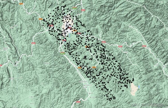
// 在图上显示GEDI数据
Map.addLayer(dataset,
    {min: 10, max: 250, palette: '440154,414387,2a788e,23a884,7ad151,fde725'},
    'Mean Biomass');
// 训练样本选择
var points = dataset.sample({
   region: roi,
   scale: 100,
   numPixels: 1000, 
   geometries: true});
// 打印信息
print(points.size());
print(points.limit(10));
Map.addLayer(points);

2. 加载两种SAR数据

var dataset = ee.ImageCollection('JAXA/ALOS/PALSAR/YEARLY/SAR')
  .filter(ee.Filter.date('2018-10-30', '2020-10-30'));
var sarHh = dataset.select('HH');
var sarHv = dataset.select('HV');
var sarHh2Vis = {
  min: 0.0,
  max: 10000.0,
};
var sarHv2Vis = {
  min: 0.0,
  max: 10000.0,
};
var clipImage = function(image) {
  return image.clip(roi);
};
var HH = sarHh.map(clipImage);
var HV = sarHv.map(clipImage);
Map.addLayer(HH, sarHh2Vis, 'SAR HH (clipped)');
Map.addLayer(HV, sarHv2Vis, 'SAR HV (clipped)');
var HH = HH.first();
var HV = HV.first();
//加载Sentinel-1 SAR数据
var S1 =  ee.ImageCollection('COPERNICUS/S1_GRD')
.filter(ee.Filter.listContains('transmitterReceiverPolarisation', 'VH'))
.filter(ee.Filter.listContains('transmitterReceiverPolarisation', 'VV'))
.filter(ee.Filter.eq('instrumentMode', 'IW'))
.filterBounds(roi)
.filterDate('2018-10-30', '2020-10-30')
.select(['VV','VH'])
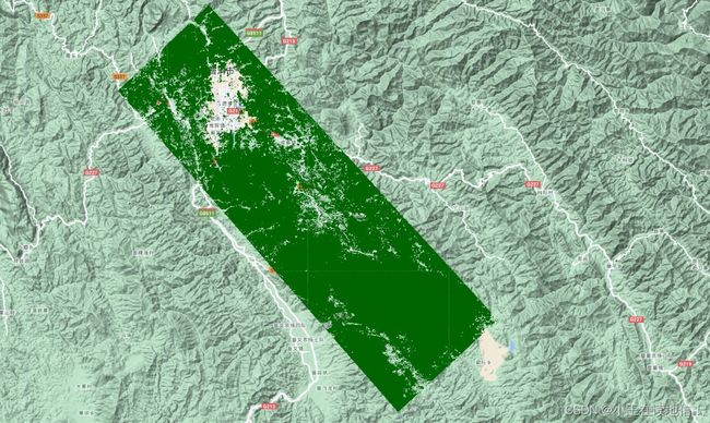
//对SAR数据的预处理进行转db值，应用滤波算法，其中还包括图像运算、核函数应用、均值计算、方差计算、梯度计算等等。下图显示了一张应用预处理完的PALSAR-2 HV极化方式的图像

3. 加载Sentinel-2数据以及其他辅助数据（SRTM-DEM、降水量数据、森林掩模数据以及森林类型数据）

//加载SRTM-DEM,裁剪SRTM-DEM,投影重采样，计算坡度,投影坡度
var SRTM = ee.Image("USGS/SRTMGL1_003");
var elevation = SRTM.clip(roi);
var elevation = elevation.reproject({crs: 'EPSG:32749',scale: 30}); 
print('Projection, crs, and crs_transform:', elevation.projection());
var slope = ee.Terrain.slope(SRTM).clip(roi);
var slope = slope.reproject({crs: 'EPSG:32749',scale: 30}); 
print('Projection, crs, and crs_transform:', slope.projection());
//加载森林掩模数据
var dataset = ee.ImageCollection("ESA/WorldCover/v100").first();
var ESA_LC_2020 = dataset.clip(roi);
var forest_mask = ESA_LC_2020.updateMask(
  ESA_LC_2020.eq(10) );
var trees = {bands: ['Map'],};
Map.addLayer(forest_mask, trees, "Trees");
//加载均降水量数据，并裁剪到感兴趣区域
var dataset = ee.ImageCollection('UCSB-CHG/CHIRPS/DAILY')
  .filter(ee.Filter.date('2018-10-30', '2020-10-30'));
var precipitation = dataset.select('precipitation');
var clippedPrecipitation = precipitation.map(function(image) {
  return image.clip(roi);
});
var rainMean = clippedPrecipitation.mean();
//加载森林类型数据(常绿林、落叶林、混交林)
var dataset = ee.Image('COPERNICUS/Landcover/100m/Proba-V-C3/Global/2019')
  .select('discrete_classification');
var foresttype = dataset.clip(roi);
Map.centerObject(roi, 10); 
Map.addLayer(foresttype, {}, 'Clipped Land Cover');
//加载Sentinel-2多光谱数据
var s2 = ee.ImageCollection("COPERNICUS/S2_SR");
var filtered = s2
  .filter(ee.Filter.date('2018-10-30', '2020-10-30'))
  .filter(ee.Filter.lt('CLOUDY_PIXEL_PERCENTAGE',10))
  .filter(ee.Filter.bounds(roi))
//对哨兵2的预处理包括了去云和中值合成等。下图显示了一张森林掩模图和森林类型图

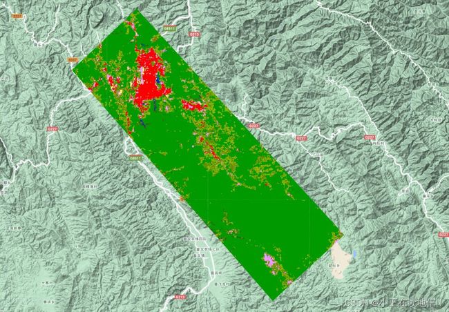
4. 中值合成以及参数运算

///哨兵1及PALSAR-2极化组合特征计算//
//1.vv+vh
var VVProductVH = combinedband.expression('VV+VH', {
    'VV' : combinedband.select('VV'),
    'VH' : combinedband.select('VH')
  }).rename('VVProductVH');
//2.vh-vv
var VHQuotientVV = combinedband.expression('VH-VV', {
    'VV' : combinedband.select('VV'),
    'VH' : combinedband.select('VH')
  }).rename('VHQuotientVV');
//3.HH/HV
var HHHV = combinedband.expression('HH/HV', {
    'HH' : combinedband.select('HH'),
    'HV' : combinedband.select('HV')
  }).rename('HH/HV');

///哨兵2植被指数计算//
//1. RVI
var rvi = combinedband.expression('NIR / RED', {
    'NIR' : combinedband.select('B8'),
    'RED' : combinedband.select('B4')
  }).rename('rvi');
//2. DVI
var dvi = combinedband.expression('NIR - RED', {
    'NIR' : combinedband.select('B8'),
    'RED' : combinedband.select('B4')
  }).rename('dvi');
//4.SAVI
var savi = combinedband.expression(
    '1.5 * (NIR - RED) /8* (NIR + RED + 0.5)', {
      'NIR': combinedband.select('B8').multiply(0.0001),
      'RED': combinedband.select('B4').multiply(0.0001),
}).rename('savi');
//5.MTCI
var mtci = combinedband.expression('(RE2 - RE1)/ (RE1 - Red)', {
    'RE2': combinedband.select('B6'),
    'RE1': combinedband.select('B5'),
     'Red': combinedband.select('B4'),
    }).rename('mtci');
//6.GNDVI
var gndvi =combinedband.expression('(RE3-Green)/(RE3+Green)', {
    'RE3': combinedband.select('B7').multiply(0.0001),
    'Green': combinedband.select('B3').multiply(0.0001),
    }).rename('gndvi');
//7.WDVI
var wdvi =combinedband.expression('NIR - 0.5*RED',{
    'NIR': combinedband.select('B8').multiply(0.0001),
    'RED': combinedband.select('B4').multiply(0.0001),
     }).rename('wdvi'); 
//8.IPVI
var ipvi=combinedband.expression('NIR/(NIR + RED )',{
    'NIR': combinedband.select('B8').multiply(0.0001),
    'RED': combinedband.select('B4').multiply(0.0001),
     }).rename('ipvi'); 
//9.NDI45
var ndi45 =combinedband.expression('(RE1-RED)/(RE1+RED)',{
    'RE1': combinedband.select('B5'),
     'RED': combinedband.select('B4'),
    }).rename('ndi45');
//10.IRECI
var ireci =combinedband.expression('(RE3-RED)/(RE1/RE2)',{
    'RE3': combinedband.select('B7'),
    'RED': combinedband.select('B4'),
    'RE1': combinedband.select('B5'),
    'RE2': combinedband.select('B6'),
}).rename('ireci'); 
//11.TSAVI
var tsavi =combinedband.expression('0.5* (NIR - 0.5*RED-0.5) / (0.5*NIR + RED -0.15 )',{
    'NIR': combinedband.select('B8').multiply(0.0001),
    'RED': combinedband.select('B4').multiply(0.0001),
}).rename('tsavi');

//12.ARVI
var arvi =combinedband.expression('(NIR-(2*RED-BLUE))/(NIR+(2*RED-BLUE))',{
    'NIR': combinedband.select('B8').multiply(0.0001),
    'RED': combinedband.select('B4').multiply(0.0001),
    'BLUE':combinedband.select('B2').multiply(0.0001),
}).rename('arvi');
//PALSAR-2纹理特征
var SS = s2bands.select('HH', 'HV').toInt32().glcmTexture().select(p2Bands)
//参数的计算包括了很多种，常用的植被指数以及纹理地形因子等等，以上只展示了部分运算。

5. 调用GEE的随机森林分类器并显示重要性以及拟合精度等

//运行 RF 分类器
var classifier = ee.Classifier.smileRandomForest(100, null, 1, 0.5, null, 0).setOutputMode('REGRESSION')
    .train({
      features: trainingData, 
      classProperty: 'MU', 
      inputProperties: bands
    });
print(classifier);
//创建的分类器对图像进行分类
var regression = selectbands.classify(classifier, 'predicted');
print(regression);
//创建图例的结构和其他美化细节


// Create the panel for the legend items.
var legend = ui.Panel({
  style: {
    position: 'bottom-left',
    padding: '8px 15px'
  }
});

// Create and add the legend title.
var legendTitle = ui.Label({
  value: 'Legend',
  style: {
    fontWeight: 'bold',
    fontSize: '18px',
    margin: '0 0 4px 0',
    padding: '0'
  }
});
legend.add(legendTitle);

// create the legend image
var lon = ee.Image.pixelLonLat()
  .select('latitude');
var gradient = lon.multiply((viz.max - viz.min) / 100.0)
  .add(viz.min);
var legendImage = gradient.visualize(viz);

// create text on top of legend
var panel = ui.Panel({
  widgets: [
    ui.Label(viz['max'])
  ],
});

legend.add(panel);

// create thumbnail from the image
var thumbnail = ui.Thumbnail({
  image: legendImage,
  params: {
    bbox: '0,0,10,100',
    dimensions: '10x200'
  },
  style: {
    padding: '1px',
    position: 'bottom-center'
  }
});

// add the thumbnail to the legend
legend.add(thumbnail);

// create text on top of legend
var panel = ui.Panel({
  widgets: [
    ui.Label(viz['min'])
  ],
});

legend.add(panel);
Map.add(legend);

// Zoom to the regression on the map
Map.centerObject(roi, 11);
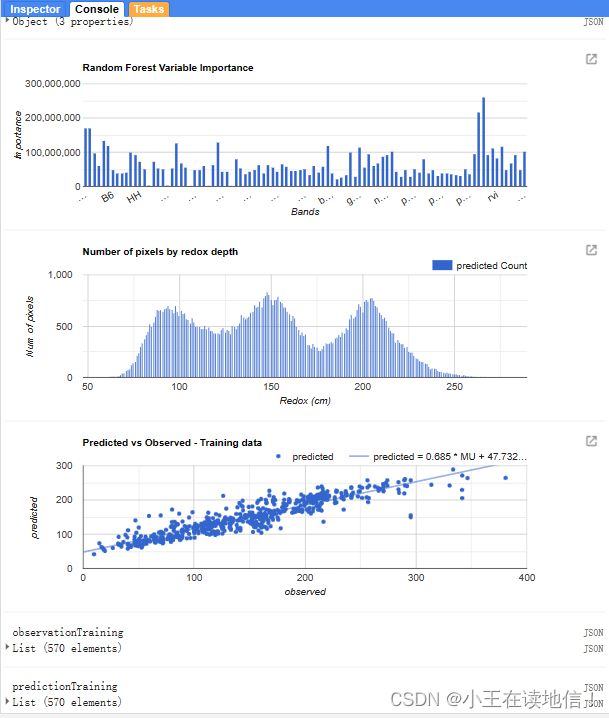
//可视化评估工具
// Get variable importance
var dict = classifier.explain();
print("Classifier information:", dict);
var variableImportance = ee.Feature(null, ee.Dictionary(dict)
  .get('importance'));
// Make chart, print it
var chart =
  ui.Chart.feature.byProperty(variableImportance)
  .setChartType('ColumnChart')
  .setOptions({
    title: 'Random Forest Variable Importance',
    legend: {
      position: 'none'
    },
    hAxis: {
      title: 'Bands'
    },
    vAxis: {
      title: 'Importance'
    }
  });
print(chart);
//直方图
var options = {
  lineWidth: 1,
  pointSize: 2,
  hAxis: {
    title: 'Redox (cm)'
  },
  vAxis: {
    title: 'Num of pixels'
  },
  title: 'Number of pixels by redox depth'
};
var regressionPixelChart = ui.Chart.image.histogram({
    image: ee.Image(regression),
    region: roi,
    scale:100
  })
  .setOptions(options);
print(regressionPixelChart);
//预测值和真实值的散点图

// Get predicted regression points in same location as training data
var predictedTraining = regression.sampleRegions({
  collection: trainingData,
  scale:100,
  geometries: true,
  projection:'EPSG:4326'
});
// Separate the observed (canopy) and predicted (regression) properties
var sampleTraining = predictedTraining.select(['MU', 'predicted']);
// Create chart, print it
var chartTraining = ui.Chart.feature.byFeature({features:sampleTraining, xProperty:'MU', yProperties:['predicted']})
  .setChartType('ScatterChart')
  .setOptions({
    title: 'Predicted vs Observed - Training data ',
    hAxis: {
      'title': 'observed'
    },
    vAxis: {
      'title': 'predicted'
    },
    pointSize: 3,
    trendlines: {
      0: {
        showR2: true,
        visibleInLegend: true
      },
      1: {
        showR2: true,
        visibleInLegend: true
      }
    }
  });
print(chartTraining);
//计算均方根误差 (RMSE)

// Get array of observation and prediction values 
var observationTraining = ee.Array(sampleTraining.aggregate_array('MU'));
var predictionTraining = ee.Array(sampleTraining.aggregate_array('predicted'));
print('observationTraining', observationTraining)
print('predictionTraining', predictionTraining)
var residualsTraining = observationTraining.subtract(predictionTraining);
print('residualsTraining', residualsTraining)
// Compute RMSE with equation, print it
var rmseTraining = residualsTraining.pow(2)
  .reduce('mean', [0])
  .sqrt();
print('Training RMSE', rmseTraining);
//验证数据执行类似的评估，以了解我们的模型在未用于训练它的数据上的表现如何
var predictedValidation = regression.sampleRegions({
  collection: validationData,
  scale:100,
  geometries: true
});
// Separate the observed (canopy) and predicted (regression) properties
var sampleValidation = predictedValidation.select(['MU', 'predicted']);
// Create chart, print it 
var chartValidation = ui.Chart.feature.byFeature(sampleValidation, 'predicted', 'MU')
  .setChartType('ScatterChart')
  .setOptions({
    title: 'Predicted vs Observed - Validation data',
    hAxis: {
      'title': 'predicted'
    },
    vAxis: {
      'title': 'observed'
    },
    pointSize: 3,
    trendlines: {
      0: {
        showR2: true,
        visibleInLegend: true
      },
      1: {
        showR2: true,
        visibleInLegend: true
      }
    }
  });
print(chartValidation);

var observationValidation = ee.Array(sampleValidation.aggregate_array('MU'));
var predictionValidation = ee.Array(sampleValidation.aggregate_array('predicted'));

var residualsValidation = observationValidation.subtract(predictionValidation);
// Compute RMSE with equation, print it
var rmseValidation = residualsValidation.pow(2)
  .reduce('mean', [0])
  .sqrt();
print('Validation RMSE', rmseValidation);

6. 展示反演图像及部分图表
   
   

结语

使用GEDI协同多源数据进行生物量反演具有很多优点，高空间分辨率：GEDI可以提供高分辨率的地球表面高度信息。与传统的遥感数据相比，GEDI的空间分辨率更高，可以更准确地捕捉到不同植被类型和结构的细微差异。这对于精确估计生物量非常重要。
全球覆盖范围：GEDI是一项全球性的任务，旨在对全球范围内的植被进行监测和评估。通过与其他遥感数据源结合使用，如卫星影像和地面观测数据，可以实现全球范围内的生物量估算。这有助于更全面地了解地球各地的植被生长情况。GEDI可以与其他遥感数据源协同工作，例如雷达和光学传感器数据。通过将GEDI的高空间分辨率高度数据与其他传感器提供的光谱、纹理等信息相结合，可以获得更全面的植被结构和生物量估计。这种多源数据协同可以提高反演结果的准确性和可靠性。
非侵入性测量：GEDI使用激光脉冲进行测量，不需要直接接触植被或土地表面。这使得GEDI能够对不同地形和植被类型进行非侵入性的生物量估算。相比于传统的野外调查方法，GEDI提供了更高效、更全面的数据收集方式。
时间序列观测：GEDI提供了连续的观测能力，可以获取不同时间点上的植被结构信息。这种时间序列观测能力对于研究植被动态变化和监测长期生态系统变化非常有价值。结合多源数据进行时间序列分析，可以揭示植被生物量的季节性和年际变化趋势。
文章只展示部分代码，因为完整的代码，对一些细节要求更加复杂，文中只提供一个GEE反演的框架。利用GEDI数据系统多种数据源的反演方法未来肯定会使得对地观测变得更简单，相信在不久的将来，实现大区域高分辨率的森林生物量估测将变得越来越便捷！