机器学习入门笔记1
目前主要跟着B站的2022吴恩达机器学习课程并完成相应的练习作业
文章目录
- 基础知识
-
- Applications
- Definition
-
- Supervised learning
- Unsupervised learning
- Linear Regression Model
- ★ \bigstar ★ Gradient descent algorithm
- Python学习
-
- 科普
- 为什么选择Python
- 编程基础
-
- 变量和简单数据类型
-
- 变量的规则
- 变量的输入
- 变量的格式化输出
- 字符串
- 数字型
-
- 整型( i n t int int)和浮点数( f l o a t float float)
- 布尔型( b o o l bool bool)
- 复数型( c o m p l e x complex complex)
- 机器学习相关代码
-
- 定义模型函数
- 定义代价函数
- 定义梯度函数
- 梯度下降算法
- 单一特征的线性回归
- 问题
- 学习资料
基础知识
Applications
Machine Learning is the science of getting computers to learn with being explicitly programmed. As a sub-field of AI, it is used to build intelligent machines. There are a few things that we could program a machine to do, such as how to find shortest path from A to B in GPS, perform web search, recognize human speech, diagnose diseases from X-rays or build a self-driving car. The one way we know how to do these things is to have a machine learn to do it by itself. ML also can work on the applications In the factory, large-scale agriculture, health care, e-commerce, and other problems. Many people have had an dream of building intelligent machines, this above AI applications research in one aspect can be called AGI or Artificial General Intelligent, a goal that get close toward by using learning algorithms.
Definition
How to actually develop a practical, valuable machine learning system.*
Supervised learning
Learn from data labeled with the giving ‘right answers’; used most; rapid advancement.
{ R e g r e s s i o n : l e a r n t o p r e d i c t i n p u t , o u t p u t , X t o Y m a p p i n g , a n u m b e r o r i n f i n i t e l y m a n y p o s s i b l e o u t p u t s C l a s s i f i c a t i o n : p r e d i c t c a t e g o r i e s , s m a l l n u m b e r o f p o s s i b l e o u t p u t s \begin{cases} \nonumber Regression &: \,learn\;to \;predict \;input, \;output,\; X \;to\; Y\; mapping, \;a \;number\; or\; infinitely\; many \;possible\; outputs\\ Classification &: \,predict \;categories, \;small \;number\; of\; possible \;outputs \end{cases} {RegressionClassification:learntopredictinput,output,XtoYmapping,anumberorinfinitelymanypossibleoutputs:predictcategories,smallnumberofpossibleoutputs
Unsupervised learning
Find something interesting in unlabeled data; data only comes with inputs; algorithm has to find structure in the data.
{ C l u s t e r i n g : g r o u p s i m i l a r d a t a p o i n t s t o g e t h e r A n o m a l y d e t e c t i o n : f i n d u n u s u a l d a t a p o i n t s D i m e n s i o n a l i t y r e d u c t i o n : c o m p r e s s d a t a u s i n g f e w e r n u m b e r s \begin{cases} \nonumber Clustering &: \,group \;similar\; data \,points\; together\\ Anomaly \,detection &: \; find\; unusual \;data\; points\\ Dimensionality \;reduction &: \; compress \;data \;using\; fewer\;numbers \end{cases} ⎩ ⎨ ⎧ClusteringAnomalydetectionDimensionalityreduction:groupsimilardatapointstogether:findunusualdatapoints:compressdatausingfewernumbers
Linear Regression Model
With one variable: one of most important thing
Construct a cost function
Prediction function :
f w , b ( x ( i ) ) = ( w ⋅ x (i) + b ) \begin{equation} \nonumber f_{w,b}(x^{(i)})=(w \cdot x^\text{(i)}+b) \end{equation} fw,b(x(i))=(w⋅x(i)+b)
where, i i i is the number of examples;
x ( i ) x^{(i)} x(i)is input value in the i i i-th sample;
w w w is weight model parameter;
b b b is bias model parameter.
Cost function :
J ( w , b ) = 1 2 m ∑ i = 1 m ( f w , b ( x ( i ) ) − y (i) ) 2 = 1 2 m ∑ i = 1 m ( w ⋅ x ( i ) + b − y ( i ) ) 2 \begin{aligned} \nonumber J(w,b)&= \frac {1} {2m} \sum_{i=1}^{m}(f_{w,b}(x^{(i)})-y^ \text{(i)})^2\\ &=\frac{1}{2m} \sum_{i=1}^{m}(w \cdot x^{(i)} +b-y^{(i)})^2 \end{aligned} J(w,b)=2m1i=1∑m(fw,b(x(i))−y(i))2=2m1i=1∑m(w⋅x(i)+b−y(i))2
where, y ( i ) y^{(i)} y(i) is target value in the i i i-th sample.
Goal :
arg min w J ( w ) \nonumber \arg\min_{w} J(w) argwminJ(w)
General case :
arg min w , b J ( w , b ) \nonumber \arg\min_{w,b} J(w,b) argw,bminJ(w,b)
★ \bigstar ★ Gradient descent algorithm
The gradient of cost function w.r.t w w w and b b b :
∂ ∂ w J ( w , b ) = ∂ ∂ w 1 2 m ∑ i = 1 m ( f w , b ( x ( i ) ) − y (i) ) 2 = ∂ ∂ w 1 2 m ∑ i = 1 m ( w ⋅ x ( i ) + b − y ( i ) ) 2 = 1 m ∑ i = 1 m ( f w , b ( x ( i ) ) − y ( i ) ) x ( i ) ∂ ∂ b J ( w , b ) = ∂ ∂ b 1 2 m ∑ i = 1 m ( w ⋅ x ( i ) + b − y ( i ) ) 2 = 1 m ∑ i = 1 m ( f w , b ( x ( i ) ) − y ( i ) ) \begin{equation} \begin{aligned} \nonumber \frac {\partial} {\partial w} J(w,b)&= \frac {\partial} {\partial w}\frac {1} {2m} \sum_{i=1}^{m}(f_{w,b}(x^{(i)})-y^ \text{(i)})^2 \\ &=\frac {\partial} {\partial w}\frac{1}{2m} \sum_{i=1}^{m}(w \cdot x^{(i)} +b-y^{(i)})^2\\ &={1 \over m} \sum_{i=1}^{m}(f_{w,b}(x^{(i)})-y^{(i)})x^{(i)}\\ \frac{\partial}{\partial b} J(w,b)&= \frac {\partial} {\partial b}\frac{1}{2m} \sum_{i=1}^{m}(w \cdot x^{(i)} +b-y^{(i)})^2\\ &=\frac {1}{m}\sum_{i=1}^{m}(f_{w,b}(x^{(i)})-y^{(i)}) \end{aligned} \end{equation} ∂w∂J(w,b)∂b∂J(w,b)=∂w∂2m1i=1∑m(fw,b(x(i))−y(i))2=∂w∂2m1i=1∑m(w⋅x(i)+b−y(i))2=m1i=1∑m(fw,b(x(i))−y(i))x(i)=∂b∂2m1i=1∑m(w⋅x(i)+b−y(i))2=m1i=1∑m(fw,b(x(i))−y(i))
Repeat until convergence : Update w w w and b b b simultaneously
w = w − α ∂ ∂ w J ( w , b ) = w − α 1 m ∑ i = 1 m ( f w , b ( x ( i ) ) − y ( i ) ) x ( i ) b = b − α ∂ ∂ b J ( w , b ) = b − α 1 m ∑ i = 1 m ( f w , b ( x ( i ) ) − y ( i ) ) \begin{equation} \begin{aligned} \nonumber w&= w-\alpha \frac {\partial} {\partial w} J(w,b)\\ &=w-\alpha \frac{1}{m}\sum_{i=1}^{m}(f_{w,b}(x^{(i)})-y^{(i)})x^{(i)}\\ b&= b-\alpha \frac{\partial}{\partial b} J(w,b)\\ &=b-\alpha\frac{1}{m}\sum_{i=1}^{m}(f_{w,b}(x^{(i)})-y^{(i)}) \end{aligned} \end{equation} wb=w−α∂w∂J(w,b)=w−αm1i=1∑m(fw,b(x(i))−y(i))x(i)=b−α∂b∂J(w,b)=b−αm1i=1∑m(fw,b(x(i))−y(i))
*where, α \alpha α is learning rate.
Python学习
科普
Python的创始人为吉多·范罗苏姆(Guido van Rossum ),1991年,第一个Python解释器诞生,它用C语言实现,并能够调用C语言的库文件。
计算机不能直接理解任何除了机器语言之外的语言,必须将程序员所写的程序语言翻译成机器语言,计算机才能执行程序。
编译器:将其他语言翻译成机器语言的工具。编译器翻译的方式有两种:编译和解释,两者区别在于翻译时间点的不同。(解释器:编译器以解释方式运行)
编译型语言:程序在执行之前需要一个专门的编译过程,(编译器)把程序编译成为机器语言的文件,运行时不需要重新翻译,直接使用编译的结果。特点:程序执行效率高,依赖编译器,跨平台性较差,如C、C++。
解释性语言:编写的程序不进行预先编译,以文本方式存储程序代码,将代码一句一句直接运行。虽然不需要编译,但必须先解释器)逐句解释再运行程序。特点:跨平台性好,编写的代码更容易阅读、调试和扩展。
为什么选择Python
人生苦短,我用Python
Python是完全面向对象的语言(面向对象是一个思维方式,也是一门程序设计技术,解决一个问题,由谁来做,是谁怎么做,多个对象,各司其职):
⋆ \star ⋆Python中一切皆为对象,函数、模块、字符串和数字都是对象
⋆ \star ⋆完全支持继承、重载、多重继承
⋆ \star ⋆支持重载运算符,也支持泛型设计
Python拥有强大的标准库,语言的核心只包含字符串、数字、列表、字典、文件等常见类型和函数,由标准库提供了系统管理、网络通信、文本处理、数据库接口、图形系统、XML处理等额外的功能
⋆ \star ⋆Python社区由形形色色充满激情,提供了大量的第三方模块,使用方式与标准库类似,它们的功能覆盖科学计算、人工智能、机器学习、Web开发、数据库接口、图形系统多个领域
编程基础
本人将每阶段对机器学习和Python的学习进行总结,因此内容不全面且显得有点杂乱,纯记录笔记
变量和简单数据类型
在内存中创建一个变量,会包括:
- 变量的名称
- 变量保存的数据
- 变量存储数据的类型
- 变量的地址(标示)
在Python中定义变量是不需要指定类型
可分为数字型和非数字型
变量的规则
∙ \bullet ∙变量名只能包含字母、数字和下划线,可以字母或下划线打头,但不能以数字打头
∙ \bullet ∙变量名不能包含空格
∙ \bullet ∙不要将Python关键字和函数名用作变量名


∙ \bullet ∙变量名应该既简短又具有描述性
∙ \bullet ∙慎用小写字母 l 和大写字母O,容易误看成数字1和0
变量的输入
用代码获取通过键盘输入的信息,用户输入的任何内容都认为是一个字符串
如下:
#常用函数
print(x)       # 将 x 输出到控制台
type(x)        # 查看 x 的变量类型
#使用 input 实现键盘输入
str_ = input ("提示信息: ")
变量的格式化输出
如果希望输出文字信息的同时,一起输出数据,需要使用格式化操作符(%)
| 格式化字符 | 含义 |
|---|---|
| %s | 字符串 |
| %d | 有符号十进制整数,%0.6d 表示输出的整数显示位数,不足的地方使用 0 补齐 |
| %f | 浮点数, %0.2f 表示小数点后只显示两位 |
| %% | 输出% |
语法格式如下:
print('格式化字符串' % 变量1 )
print('格式化字符串' % (变量1,变量2...))
字符串
分清楚方法和函数的区别,方法是Python可以对数据执行的操作,由于方法通常需要额外的信息来完成其工作,因此每一个方法后面都跟着一对括号,当不需要额外的信息时,括号内是空的。
在Python中,字符串用引号或单引号括起:
str_ = ‘this is a string. "ada lovelace" ' # 将字符串存储到变量str_
以下为对字符串进行操作可能用到的方法:
str_.title()         # 将字符串首字母大写
str_.upper()         # 将字符串全部改为大写
str_.lower()         # 将字符串全部改为小写
str_.rstrip()        # 剔除字符串末尾的空白,不改变原变量
str_.lstrip()        # 剔除字符串开头的空白
str_.strip()         # 剔除字符串两端的空白
str3 = str1 + str2   # 使用(+)来合并或拼接字符串

# 使用非打印字符,如空格“  ”、制表符 \t、换行符 \n 来添加空白
数字型
调用函数 s t r ( ) str( ) str()或 i n t ( ) int( ) int()强制类型转换,避免类型错误
str(int_)            # 转换成字符串
int(str_)            # 转换成整数
float(str_)          # 转换成浮点数
整型( i n t int int)和浮点数( f l o a t float float)
#执行运算
2+3                  # (+),加法
3-1                  # (-),减法
2*3                  # (*),乘法
3.0/2                # (/),除法,返回 1.5
3**2                 # (**),乘方
3%2                  # (%),求模,返回余数 1
9//4                 # (//),取整,结果为 4
布尔型( b o o l bool bool)
真 T u r e Ture Ture 非零数( 1 1 1)——非零即真
假 F a l s e 0 False \quad 0 False0
复数型( c o m p l e x complex complex)
主要用于科学计算,例如:平面场问题、波动问题、电感电容等问题
机器学习相关代码
第一次发博客,为了简短内容,只记录学习中做的作业,而对于Python中的numpy库和matplotlib库,以及在做作业过程中所接触到的不认识的函数和方法,打算将在之后的笔记中不断补充
定义模型函数
# 导入所需模块
import numpy as np
import matplotlib.pyplot as plt
# 显示交互式动态数据
%matplotlib widget
plt.style.use('./deeplearning.mplstyle')
plt.style.use('seaborn-darkgrid')
# 定义模型函数
def compute_modul_output(x,w,b):
    """
    Computes the prediction of a linear model
    Args:
        x(ndarray(m,)):Data, m examples
        w,b (scalar)  : model parameters
    Returns
        y(ndarray (m,)): target values
    """
    m=x.shape[0]
    f_wb=np.zeros(m)
    for i in range(m):
        f_wb[i]= w*x[i]+b
    return f_wb
定义代价函数
#定义代价函数
def compute_cost(x,y,w,b):

    m=x.shape[0] #样本数量
    cost=0

    for i in range(m): #输入m个样本,计算代价
        f_wb = w*x[i]+b #线性方程
        cost = cost+(f_wb-y[i])**2 #误差平方求和
        total_cost = 1/(2*m)*cost  #均方误差

    return total_cost
定义梯度函数
#定义梯度函数,计算梯度
def compute_gradient(x,y,w,b):
    """
    Comopute the gradient for linear regrssion
    Args:
        x(ndarray(m,)): Data, m examples
        y(ndarray(m,)): target value
        w,b(scalar)   : model parameters
    Returns
        dj_dw (scalar): The gradient of the cost w.r.t the parameter w
        dj_db (scalar): The gradient of the cost w.r.t the parameter b
    """
    #训练样本数量
    m=x.shape[0]
    dj_dw = 0
    dj_db = 0

    for i in range(m):
        f_wb = w*x[i]+b
        #求和
        dj_dw_i = (f_wb-y[i])*x[i]
        dj_db_i = f_wb-y[i]
        dj_dw += dj_dw_i  # or dj_dw = dj_dw + f_wb-y[i]*x[i]
        dj_db += dj_db_i
        dj_dw = dj_dw / m
        dj_db = dj_db / m
    return dj_dw, dj_db
梯度下降算法
#定义梯度下降算法
def gradient_descent(x, y, w_in, b_in, alpha, num_iters, cost_function, gradient_function):
    """
    Args:
        x(ndarray(m,)) : Data, m examples
        y(ndarray(m,)) : target values
        w_in, b_in(scalar) : initial values of model parameters
        alpha (float) : learning rate
        num_iters (int): number of iterations to run gradient descent
        cost_function : function to call to produce cost
        gradient_function : function to call to produce gradient

    Returns
        w (scalar) : updated value of parameter after running gradient descent
        b (scalar) : updated value of parameter after running gradient descent
        J_history (list) : history of cost values
        p_history (list) : history of parameters[w,b]
        """
    w = copy.deepcopy(w_in) #作为独立变量,避免全局编辑
    #建立一个数组来保存每次迭代的代价J以及w,用于后续画图
    J_history = []
    p_history = []
    b = b_in
    w = w_in

    for i in range (num_iters):
        dj_dw, dj_db = gradient_function (x, y, w, b) #运用梯度函数计算梯度,并更新参数
        w = w-alpha * dj_dw #改变权重和bias
        b = b-alpha * dj_db

    #每次迭代保存cost & J
        if i<100000:   #防止资源枯竭
            J_history.append ( cost_function(x, y, w, b))
            p_history.append ([w,b])
     #每隔10次就打印一次成本,如果<10,则打印相同次数的迭代。
        if i% math.ceil(num_iters/10) == 0:  # ceil 表示返回数字的上入整数,i 是否被num_iter/10整除
            print(f"Interation {i:4} : Cost {J_history[-1]: 0.2e}",
                 f"dj_dw: {dj_dw: 0.3e}, dj_db: {dj_db: 0.3e}",
                 f"w: {w: 0.3e}, b: {b:0.5e}")

    return w, b, J_history, p_history  #返回w 和J ,w的历史数据用来绘图
单一特征的线性回归
#导入所需模块
import math, copy
import numpy as np
import matplotlib.pyplot as plt
plt.style.use('./deeplearning.mplstyle')
from lab_utils_uni import plt_house_x, plt_contour_wgrad, plt_divergence, plt_gradients
#创建数据集
x_train=np.array([1,2]) #特征输入
y_train=np.array([300,500]) #目标值
#定义代价函数
def compute_cost(x,y,w,b):

    m=x.shape[0] #样本数量
    cost=0

    for i in range(m): #输入m个样本,计算代价
        f_wb = w*x[i]+b #线性方程
        cost = cost+(f_wb-y[i])**2 #误差平方求和
        total_cost = 1/(2*m)*cost  #均方误差

    return total_cost
#定义梯度函数,计算梯度
def compute_gradient(x,y,w,b):
    """
    Comopute the gradient for linear regrssion
    Args:
        x(ndarray(m,)): Data, m examples
        y(ndarray(m,)): target value
        w,b(scalar)   : model parameters
    Returns
        dj_dw (scalar): The gradient of the cost w.r.t the parameter w
        dj_db (scalar): The gradient of the cost w.r.t the parameter b
    """
    #训练样本数量
    m=x.shape[0]
    dj_dw = 0
    dj_db = 0

    for i in range(m):
        f_wb = w*x[i]+b
        #求和
        dj_dw_i = (f_wb-y[i])*x[i]
        dj_db_i = f_wb-y[i]
        dj_dw += dj_dw_i  # or dj_dw = dj_dw + f_wb-y[i]*x[i]
        dj_db += dj_db_i
        dj_dw = dj_dw / m
        dj_db = dj_db / m
    return dj_dw, dj_db
#运行plt_gradients 查看cost &gradient 相对于w的变化,其中b=100
plt_gradients(x_train, y_train, compute_cost, compute_gradient)
plt.show()
#定义梯度下降算法
def gradient_descent(x, y, w_in, b_in, alpha, num_iters, cost_function, gradient_function):
    """
    Args:
        x(ndarray(m,)) : Data, m examples
        y(ndarray(m,)) : target values
        w_in, b_in(scalar) : initial values of model parameters
        alpha (float) : learning rate
        num_iters (int): number of iterations to run gradient descent
        cost_function : function to call to produce cost
        gradient_function : function to call to produce gradient

    Returns
        w (scalar) : updated value of parameter after running gradient descent
        b (scalar) : updated value of parameter after running gradient descent
        J_history (list) : history of cost values
        p_history (list) : history of parameters[w,b]
        """
    w = copy.deepcopy(w_in) #作为独立变量,避免全局编辑
    #建立一个数组来保存每次迭代的代价J以及w,用于后续画图
    J_history = []
    p_history = []
    b = b_in
    w = w_in

    for i in range (num_iters):
        dj_dw, dj_db = gradient_function (x, y, w, b) #运用梯度函数计算梯度,并更新参数
        w = w-alpha * dj_dw #改变权重和bias
        b = b-alpha * dj_db

    #每次迭代保存cost & J
        if i<100000:   #防止资源枯竭
            J_history.append ( cost_function(x, y, w, b))
            p_history.append ([w,b])
     #每隔10次就打印一次成本,如果<10,则打印相同次数的迭代。
        if i% math.ceil(num_iters/10) == 0:  # ceil 表示返回数字的上入整数,i 是否被num_iter/10整除
            print(f"Interation {i:4} : Cost {J_history[-1]: 0.2e}",
                 f"dj_dw: {dj_dw: 0.3e}, dj_db: {dj_db: 0.3e}",
                 f"w: {w: 0.3e}, b: {b:0.5e}")

    return w, b, J_history, p_history  #返回w 和J ,w的历史数据用来绘图
#初始化参数
w_init = 0
b_init = 0
#选择迭代次数以及设置学习速率
iterations = 10000
temp_alpha = 1.0e-2
#运行梯度下降
w_final, b_final, J_hist, p_hist = gradient_descent(x_train, y_train, w_init, b_init, temp_alpha, iterations, compute_cost, compute_gradient)
print(f"(w,b) found by gradient descent: ({w_final:1.2f}, {b_final:1.2f})")
#绘制成本与代价
fig, (ax1,ax2) = plt.subplots(1, 2, constrained_layout=True, figsize=(12,4))  #创建画布,作两幅图
ax1.plot(J_hist[:100]) #绘制0~100的数据图
ax2.plot(1000+ np.arange(len(J_hist[1000:])), J_hist[1000:]) #绘制1000~最后的数据图
ax1.set_title("Cost vs. iteration(start)")
ax2.set_title("Cost vs. iteration (end)")
ax1.set_ylabel('Cost')
ax2.set_ylabel('Cost')
ax1.set_xlabel('interation step')
ax2.set_xlabel('iteration step')
plt.show()
#预测房价
print(f"1000 sqft house prediction {w_final*1.0 + b_final: 0.1f} Thousand dollars ")
print(f"1200 sqft house prediction {w_final*1.2 + b_final: 0.1f} Thousand dollars ")
print(f"1500 sqft house prediction {w_final*1.5 + b_final: 0.1f} Thousand dollars ")
#在cost(w,b)等高线图上绘制迭代过程的cost变化显示梯度下降进展
fig, ax=plt.subplots(1,1, figsize=(12,6)) #创建画布,绘制一张一行一列,大小为12x6的图
plt_contour_wgrad(x_train, y_train, p_hist, ax)   # 绘制等高线图,调用已给辅助函数
#局部放大
fig, ax= plt.subplots(1,1, figsize=(12,4))
plt_contour_wgrad(x_train, y_train, p_hist, ax, w_range=[180, 220, 0.5], b_range=[80, 120, 0.5], contours=[1,5,10,20], resolution=0.5)
#增大学习速率
w_int=0
b_int=0 #初始化权重和bias
interations = 10
tmp_alpha = 9.0e-1 #迭代次数10次,学习速率0.9
w_final, b_final, J_hist, p_hist= gradient_descent(x_train, y_train, w_int, b_int, tmp_alpha, interations, compute_cost, compute_gradient)
#学习速率太大引起发散现象
plt_divergence(p_hist, J_hist, x_train, y_train)
plt.show()
问题
在做练习作业过程中,主要的问题是由于之前没有学习过Python,在自己敲代码时,总会出现各种错误,多亏了CSDN中各博主的帮助,才得以解决。在学习语言时,不仅要学会语言的语法,还要学会如何认识和解决错误的方法,因此记录了一部分,如下所示:
1.
注意 d e f f u n c t i o n ( ) def \;function() deffunction()内的格式
2.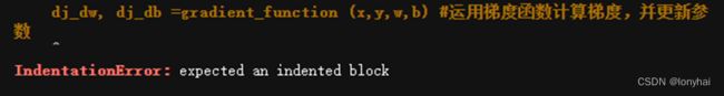 格式,注意应该缩进就缩进,如图所示:
3.
注意{}内格式,
学习资料
[1] Python编程 从入门到实践 第2版 作者: [美] 埃里克·马瑟斯(Eric Matthes)著
[2] Python大战机器学习:数据科学家的第一个小目标 作者:华校专 王正林
[3] Python编程从入门到实践笔记(超详细的精华讲解+内有2021最新版本代码)
保持专注,好奇心,以谦卑的心态不断学习,做到知行合一。