时间序列预测专项——基于Prophet的业务预测
时间序列预测专项
- 基于Prophet的业务预测
-
- 1. 趋势模型
-
- 1.1 饱和增长模型
- 1.2 分段线性模型
- 1.3 变点自动选择
- 2. 季节模型
- 3. 节假日模型
- 4. Prophet模型参数解读
- 5. Prophet模型的Python实现demo
-
- 5.1 Prophet参数介绍
- 5.2 饱和回归模型demo
- 5.3 季节模型demo
- 5.4 外生效应
- 参考资料
基于Prophet的业务预测
Prophet模型将时间序列分成三个成分:趋势项、季节项、节假日项。模型形式如下:
y ( t ) = g ( t ) + s ( t ) + h ( t ) + ε ( t ) y(t)=g(t)+s(t)+h(t)+\varepsilon(t) y(t)=g(t)+s(t)+h(t)+ε(t)
Prophet模型通过加法将趋势项、季节项、节假日项组合在一起,可以很方便地剥离出不同成分对时间序列的影响或效应。
- g ( t ) g(t) g(t)为趋势项,趋势模型用于拟合时间序列的趋势成分,对非周期性变化建模。
- s ( t ) s(t) s(t)为季节项,季节模型用于拟合周期性的变化,例如周季节性、年季节性等。
- h ( t ) h(t) h(t)为节假日项,节假日模型可以对一天或连续几天产生影响的突发事件或节假日效应进行建模。
- ε ( t ) \varepsilon (t) ε(t)为误差项,代表不能被模型识别的特异性变化。
1. 趋势模型
这里考虑两个趋势模型:饱和增长模型(回归趋势模型)和分段线性模型。
1.1 饱和增长模型
在自然经济学中,人口规模不会沿着J型曲线无限增长,最终会由于自然环境的承载力的限制而趋于饱和。在研究互联网用户增长模式时套用此模型,可以假设产品用户量也会由于入网人数(承载力)的影响而达到饱和。原始的饱和增长模型形式如下:
g ( t ) = C 1 + e x p ( − k ( t − m ) ) g(t)= \frac{C}{1+exp(-k(t-m))} g(t)=1+exp(−k(t−m))C
其中,C是承载力,代表业务指标理想中的最大值。k是增长率,m是补偿系数。
这里给出的饱和增长模型形式原始形式有两个问题。
- C是承载力,代表业务指标理想中的最大值。但C会随着时间的变化而产生变化。例如,随着入网人数的增多,承载力也会增多。
- k是增长率。业务指标的增长率也不是一成不变的。例如:新产品的发布,重大营销活动等都可能会使业务指标的趋势产生明显的变化。
为了解决第一个问题。可以引入外部数据 C ( t ) C(t) C(t),对每一时刻的指标值给定不同的承载力。
为了解决第二个问题。通过定义变点,将导致趋势改变的点放在模型中。设,有 S S S个变点,第 j j j个变点在 s j s_j sj时刻对增长率的影响为 δ j \delta_j δj,于是可以得到增长率 k ′ k^{'} k′:
k ′ = k + ∑ j : t > s j δ j = a j ( t ) T δ k^{'}=k+\sum_{j:t>s_j} \delta_j =a_j(t)^{T}\delta k′=k+j:t>sj∑δj=aj(t)Tδ
其中 a j ( t ) = { 1 t ≥ 1 0 e l s e a_j(t)=\begin{cases} 1 & t \ge1 \\ 0 & else \end{cases} aj(t)={10t≥1else.
于是,修正后的饱和趋势模型的形式如下:
g ( t ) = C ( t ) 1 + e x p ( − k ′ ( t − m ′ ) ) g(t)=\frac{C(t)}{1+exp(-k^{'}(t-m^{'}))} g(t)=1+exp(−k′(t−m′))C(t)
1.2 分段线性模型
分段线性模型的形式如下:
g ( t ) = k ′ t + ( t − m ′ ) g(t)=k^{'}t+(t-m^{'}) g(t)=k′t+(t−m′)
1.3 变点自动选择
变点可以是分析师通过经验给出的可能会导致趋势变化的日期,也可以通过给定趋势模型稀疏的先验 δ \delta δ自动识别出来一系列可能的变点。先验的 δ j \delta_j δj~ L a p l a c e ( 0 , τ ) Laplace(0, \tau ) Laplace(0,τ)。
2. 季节模型
函数的傅里叶展开,通俗理解就是一个周期为T=2L的函数可以表示为无限个简单的周期函数之和。季节模型是通过傅里叶级数去模拟时间序列的季节/周期效应。
S ( t ) = ∑ n = 1 N ( a n cos ( 2 π n t P ) + b n s i n ( 2 p i n t P ) ) S(t)=\sum_{n=1}^{N}(a_n\cos(\frac{2\pi nt}{P})+b_nsin(\frac{2pi nt}{P})) S(t)=n=1∑N(ancos(P2πnt)+bnsin(P2pint))
当考虑年季节性时 P = 365.25 P=365.25 P=365.25;考虑周季节性时 P = 7 P=7 P=7。
设 β = [ a 1 , b 1 , . . . , a N , b N ] β = [a1, b1, . . . , aN , bN ] β=[a1,b1,...,aN,bN],则 S ( t ) = X ( t ) β S(t)=X(t)\beta S(t)=X(t)β
这里 β \beta β的先验分布为 N ( 0 , σ 2 N(0,\sigma^{2} N(0,σ2)。
3. 节假日模型
不同国家有不同的传统节假日,节假日模型可以考虑不同国家的节假日效应。对于每个节假日 i i i, D i D_i Di表示其对应的日期,定义指示函数去表示时间 t t t是否为节假日日期。 κ \kappa κ为节假日的影响效应。
Z ( t ) = [ 1 ( t ∈ D 1 ) , . . . , 1 ( t ∈ D L ) ] Z(t) = [1(t ∈ D1), . . . , 1(t ∈ DL)] Z(t)=[1(t∈D1),...,1(t∈DL)]
于是,节假日模型形式为:
h ( t ) = Z ( t ) κ h(t) = Z(t)\kappa h(t)=Z(t)κ
其中 κ \kappa κ~ N o r m a l ( 0 , ν 2 ) Normal(0,\nu^{2}) Normal(0,ν2)
4. Prophet模型参数解读
τ : \tau: τ:调节趋势模型的flexibility
σ : \sigma: σ:调节季节模型的strength
5. Prophet模型的Python实现demo
5.1 Prophet参数介绍
Prophet(self, growth=u'linear', changepoints=None, n_changepoints=25,
yearly_seasonality=u'auto', weekly_seasonality=u'auto',
daily_seasonality=u'auto', holidays=None, seasonality_prior_scale=10.0,
holidays_prior_scale=10.0, changepoint_prior_scale=0.05,
mcmc_samples=0, interval_width=0.8, uncertainty_samples=1000)
- growth: String ‘linear’ or ‘logistic’
- holidays: pd.DataFrame. columns= [holiday (string) ,ds (date type), lower_window ,upper_window, prior_scale].其中lower_window,upper_window分别为节假日的左窗口和右窗口,可以同时考虑节假日的预热效应和滞后效应。prior_scale调节节假日模型强度的参数,取值越大,会越增强节假日效应;取值越小,则会减弱节假日效应。
- seasonality_prior_scale:调节季节模型的强度参数,取值越大,越能识别季节的波动;取值越小,则会减弱季节性。
- changepoint_prior_scale( τ \tau τ):调节变点自动选择灵敏度的参数。取值越大,越能得到更多的可选的变点;取值越小,则变电越少。
5.2 饱和回归模型demo
# 加载包
import pandas as pd
from fbprophet import Prophet

# DATA为prophet包里面给的示例数据
DATA = pd.read_csv(
    'data.csv',
    parse_dates=['ds'],
)

# 饱和回归模型demo
m = Prophet(growth='logistic')
N = DATA.shape[0]
DATA_history = DATA.head(N // 2).copy()
DATA_future  = DATA.tail(N // 2).copy()
history = DATA_history
future  = DATA_future

# 给定指标的floor,capacity值
history['floor'] = history['y'].min()
history['cap'] = history['y'].max()
future['floor'] = history['floor'].mean()*1.05
future['cap'] = history['cap'].mean()*1.05

# 拟合模型
m.fit(history)
fcst1 = m.predict(future)
fcst1.head()
5.3 季节模型demo
# 节假日设置
holidays = pd.DataFrame({
'ds': pd.to_datetime(['2017-01-02']),
'holiday': ['special_day'],
'prior_scale': [4.],
'lower_window':-2,
'upper_window':2
})
m = Prophet(holidays=holidays, yearly_seasonality=False)
# 添加月季节性
m.add_seasonality(name='monthly', period=30, fourier_order=5,
prior_scale=2.)
# 拟合模型
m.fit(history)
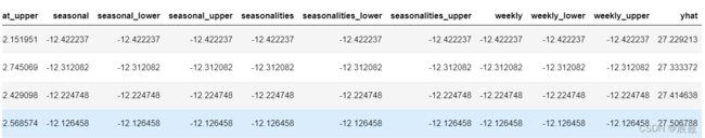
fcst2 = m.predict(future)
fcst2.head()
# 拟合值=趋势效应+节假日效应+季节效应
fcst2[['trend','holidays','seasonalities']].sum(axis=1)==fcst2['yhat']
5.4 外生效应
在实际中,运营指标之间也可能存在一定的相关性。例如:收入可能会受到客单价、客户量等因素的影响。在进行Prophet模型预测时,除了考虑趋势效应、季节效应、节假日效应,也可以同事考虑一些外生变量对运营指标的影响。add_regressor(m, name, prior.scale = NULL, standardize = 'auto' )
在原数据框中增加一列作为解释变量,当参数standardize='auto’时,这个解释变量将会被标准化(除非它是二进制),给定浮动比例参数时回归系数也就确定了,降低浮动比例会产生较大的调整,当不指定浮动比例时,默认为holidays.prior.scale的值。
m = Prophet(holidays=holidays, yearly_seasonality=False)
# 添加外生变量
m.add_regressor('binary_feature', prior_scale=0.2)
m.add_regressor('numeric_feature', prior_scale=0.5)
m.add_regressor('binary_feature2', standardize=True)
df = DATA.copy()
df['binary_feature'] = [0] * 255 + [1] * 255
df['numeric_feature'] = range(510)
df['binary_feature2'] = [1] * 100 + [0] * 410
m.fit(df)
future['binary_feature']=1
future['numeric_feature']=49
future['binary_feature2']=0
fcst3 = m.predict(future)
# 拟合值=趋势效应+节假日效应+季节效应+外生效应
fcst3[['trend','holidays','seasonalities','extra_regressors']].sum(axis=1)==fcst2['yhat']
参考资料
[1]:https://peerj.com/preprints/3190v2/
[2]: https://facebook.github.io/prophet/