MATLAB图像处理项目
一个使用MATLAB进行图像处理的项目总结,帮助理解图像处理算法和过程。
需要完成以下任务:
(1)读取并显示原始图像。
(2)对图像进行阈值操作并将其转换为二值图像。
(3)确定物体的1像素薄图像。
(4)确定图像轮廓。
(5)给图像中不同的物体赋予标签,连接方法采用4连接和8连接。
文章目录
一、项目要求
二、分步实现
(1)读取并显示原始图像
(2)对图像进行阈值操作并将其转换为二进制图像
(3)确定物体的1像素薄图像
(4)确定图像轮廓
(5)给图像中不同的物体赋予标签
总结
一、项目要求
给定一个64x64、32级的图像。这些图像显示为编码阵列,每个像素包含一个字母数字字符。这些字符的范围是0-9和A-V,对应于32级灰度。
需要完成以下任务:
(1)读取并显示原始图像。
(2)对图像进行阈值操作并将其转换为二值图像。
(3)确定物体的1像素薄图像。
(4)确定图像轮廓。
(5)给图像中不同的物体赋予标签,连接方法采用4连接和8连接。
二、分步实现
(1)读取并显示原始图像
图像均以多种图像文件格式进行组织和存储。图像中的数据可以代表性地以三种格式类型存储:未压缩格式、压缩格式和矢量格式。数字数据包含在其中一种格式的图像中,并且可以在光栅化数据之后显示图像。光栅化是将图像数据转换为像素网格的过程,该网格根据比特数确定其颜色。对于本项目中给出的图像,每个字符都被指定了相应的像素,以成功地执行图像显示。
本例中,图像中的字母A-V被适当地映射到相应的像素值,以适应项目表中建议的灰度级32的范围。
代码实现:
%% 1. Open and display the original image
chromo = fopen('chromo.txt');              % open the file
lf = newline;                              % line feed character,newline == char(10)
cr = char(13);                             % carriage return character
ch = fscanf(chromo,[cr lf '%c'],[64, 64]); % ignore linefeed and carriage return, put in 64X64 matrix
fclose(chromo);                            % close the file

ch = ch';                                  % transpose since fscanf returns column vectors
ch(isletter(ch)) = ch(isletter(ch)) - 55;  % convert letters A‐V to their corresponding values in 32 gray levels
ch(ch >= '0' & ch <= '9') = ch(ch >= '0' & ch <= '9') - 48; % convert number 0‐9 to their corresponding values in 32 gray levels
ch = uint8(ch);                            % uint8 in range(0-255), 8-bit unsigned integer, 1 byte
img = ch;
% the ASCII value of A is 65, after subtracting 55 the value of A is 10, and so on

% another method
% char2num = [zeros(1,'0'-1), 0:9, zeros(1,'A'-'9'-1), (0:('V'-'A')) + 10];
% img = 32*mat2gray(char2num(ch'),[0 32]);   % transpose matrix and convert to grayscale image

imshow(img,[0 32],'InitialMagnification','fit');
title('Original image:');
% display the image, need to define [0 32], because always read the image with default grayscale of 255
% display the appropriate size image
打开文件后,char(10)处理换行符(newline命令效果相同),char(13)回车字符。忽略所有的换行字符和回车字符,放在64X64矩阵中。
显示图像有两种代码方法:
(1)矩阵首先转置,因为fscanf返回列向量。之后将字母A-V、数字0-9转换为其在32个灰度等级中的相应值。A的ASCII值是65,减去55后A的值是10;0的ASCII值是48,减去48后0的值是0,以此类推。uint8命令将范围规定在0-255,即8位无符号整数,也就是1个字节。
(2)另一种比较简练,直接调用char2num函数,实现逻辑相同。
最后要把图像显示出来,需要定义[0 32]的范围,因为总是以默认的255灰度来读取图像。同时把图像调整到适当大小。

(2)对图像进行阈值操作并将其转换为二进制图像
图像阈值处理是许多图像处理和计算机视觉应用中的关键步骤,它可以通过将灰度图像转换成二值图像,将感兴趣的对象从背景中分离出来。图像阈值处理通常作为预处理步骤,用于物体识别、边缘检测和分割任务等等。这里采用了两种阈值方法:基本全局阈值和Otsu方法。具体的阈值计算方法请参考之前的文章。
二进制机器视觉与阈值方法
主程序代码:
%% 2. Threshold the image and convert it into binary image
figure();

subplot(1,2,1);
BGT = Basic_Global_Threshold_func(img);
imshow(img > BGT,'InitialMagnification','fit');   % Basic global threshold image
title(['Basic Global Thresholding at: ', num2str(BGT)]);

subplot(1,2,2);
Otsu = Otsu_Threshold_func(img);
imshow(img > Otsu,'InitialMagnification','fit');  % Otsu method threshold image
title(['Otsu Thresholding at: ', num2str(Otsu)]);
分别调用了两个阈值处理函数。首先是基本全局阈值,代码实现如下:
function BGT = Basic_Global_Threshold_func(img)
% Basic Global Thresholding Calculation

T = 20; % define initial estimate value
T_0 = 0;

G1 = img >  T;
G2 = img <= T;           % use T to get 2 groups of pixels
mean_1 = mean(img(G1));
mean_2 = mean(img(G2));  % get the mean value

while abs(T-T_0) > (10^-12)  % set the tolerance
    T_0 = T;
    T   = (mean_1 + mean_2)/2;
    G1  = img >  T;
    G2  = img <= T;
    mean_1 = mean(img(G1));
    mean_2 = mean(img(G2));
end

BGT = T;
end
定义20为初始阈值,确定基本全局阈值。另一种采用Otsu方法,代码实现:
function Otsu = Otsu_Threshold_func(img)
% Otsu's Method Thresholding

% get the histogram, scan all pixels
intensity_level = zeros(1,32);
sz = size(img);
for b = 1:sz(1)
    for j = 1:sz(2)
        z = img(b,j);
        intensity_level(z+1) = intensity_level(z+1) + 1;
    end
end

% set the maximum variance, total pixels and sigma value
maximum_variance = 10^-12;
total_pixels = sum(intensity_level);
sigma = zeros(1,32);

% probability levels of pixels
probability_levels = intensity_level / total_pixels;

% devide and calculate
for b = 1:16
    p1 = sum(probability_levels(1:b));
    p2 = sum(probability_levels(b+1:end));
    m1 = dot(0:b-1,probability_levels(1:b))   / p1;
    m2 = dot(b:31,probability_levels(b+1:32)) / p2;
    sigma(b) = sqrt(p1*p2*((m1-m2)^2));

end
maximum_variance = max(sigma);
Otsu = find(sigma == maximum_variance)-1;

end
显示阈值处理之后的结果如下:

(3)确定物体的1像素薄图像
图像细化是一种重要的图像处理技术,通过将物体的宽度减小到单个像素的厚度来简化二进制图像,广泛应用在模式识别、计算机视觉和图像分析等场景中。在本例中采用Zhang-Suen算法来处理由上一步经两种阈值处理技术生成的二值图像。具体的算法处理过程请参考之前的文章。
图像细化和骨架提取
主程序代码实现,分别使用两种阈值来调用Zhang-Suen算法函数:
%% 3.Determine a one-pixel thin image of the objects
figure();

subplot(1,2,1);
zhang_suen_algorithm(img < BGT);
title('Thinned image by Zhang Suen Algorithm with Basic Global Thresholding:');
subplot(1,2,2);
zhang_suen_algorithm(img < Otsu);
title('Thinned image by Zhang Suen Algorithm with Otsu Thresholding:');
算法实现函数:
function zhang_suen_algorithm(binary_img)
    % get the binary image
    [m, n] = size(binary_img);             % get the image size
    img = padarray(binary_img, [1 1], 0);  % padding the image
    en = 0;   % define the enable signal
    [obj_row,obj_col] = find(binary_img == 1);

    while en ~= 1
        tmp_img = img;

        % Step 1
        for p = 2:length(obj_row)
            % for b = 2:length(obj_cols)

            rand_array = randperm(length(obj_row));
            i = obj_row(rand_array(1));
            j = obj_col(rand_array(1));

            if i == 1 || i == m
                continue
            elseif j == 1 || j == n
                continue
            end

            % get the pixel, order is: P1,P2,P3...P8,P9,P2
            core_pixel  = [img(i,j)     img(i-1,j)   img(i-1,j+1) ...
                           img(i,j+1)   img(i+1,j+1) img(i+1,j)   ...
                           img(i+1,j-1) img(i,j-1)   img(i-1,j-1) ...
                           img(i-1,j)];

            A_P1 = 0;    % value change times
            B_P1 = 0;    % non zero neighbors
            for k = 2:9
                if core_pixel (k) < core_pixel (k+1)
                    A_P1 = A_P1 + 1;
                end
                if core_pixel (k) == 1
                    B_P1 = B_P1 + 1;
                end
            end

            if ((core_pixel(1) == 1)                                    &&...
                   (A_P1 == 1)                                          &&...
                   ((B_P1 >= 2) && (B_P1 <= 6))                         &&...
                   (core_pixel(2) * core_pixel(4) * core_pixel(6) == 0) &&...
                   (core_pixel(4) * core_pixel(6) * core_pixel(8) == 0))
               img(i, j) = 0;
            end
        end

        % when previous image is equal to current image, break the loop
        en = isequal(tmp_img, img);
        if en
           break
        end

 %---------------------------------------------------------------------------------
        tmp_img = img;
        % Step 2
        for p = 2:length(obj_row)
            % for b = 2:length(obj_cols)

            rand_array=randperm(length(obj_row));
            i = obj_row(rand_array(1));
            j = obj_col(rand_array(1));

            if i== 1 || i == m
                continue
            elseif j==1 || j== n
                continue
            end

            core_pixel  = [img(i,j)     img(i-1,j)   img(i-1,j+1) ...
                           img(i,j+1)   img(i+1,j+1) img(i+1,j)   ...
                           img(i+1,j-1) img(i,j-1)   img(i-1,j-1) ...
                           img(i-1,j)];

            A_P1 = 0;
            B_P1 = 0;
            for k = 2:9
                if core_pixel (k) < core_pixel (k+1)
                    A_P1 = A_P1 + 1;
                end
                if core_pixel (k) == 1
                    B_P1 = B_P1 + 1;
                end
            end

            if ((core_pixel(1) == 1)                                    &&...
                   (A_P1 == 1)                                          &&...
                   ((B_P1 >= 2) && (B_P1 <= 6))                         &&...
                   (core_pixel(2) * core_pixel(4) * core_pixel(8) == 0) &&...
                   (core_pixel(2) * core_pixel(6) * core_pixel(8) == 0))
               img(i, j) = 0;
            end
        end

        % when previous image is equal to current image, break the loop
        en = isequal(tmp_img, img);
        if en
           break
        end
    end

    img_thinned = [m,n];
    img = 1 - img;
    for i = 2:m+1
        for j = 2:n+1
            img_thinned(i-1, j-1) = img(i,j);
        end
    end

    imshow(img_thinned,'InitialMagnification','fit');

end
显示处理结果:

对于细化过程来说,选择合适的阈值处理方法至关重要,因为它会显著影响处理过程的结果,而阈值化方法的选择则取决于具体应用和输入图像的特征。
(4)确定图像轮廓
提取二值图像中物体的轮廓是物体识别、分割和形状分析等各种图像处理任务中必不可少的一步。在这里我提供的代码通过考虑二值图像的每一行和每一列,实现了一种直接的轮廓提取方法。该方法会扫描输入二值图像的行和列,并将每个像素与其相邻像素进行比较。如果一个像素是前景像素(foreground pixel,值为 1),而其左侧、右侧、顶部或底部有一个背景像素(background pixel,值为 0),则该像素被视为轮廓像素。
处理过程如下:
a. 将每一行的像素与其左右邻近像素进行比较。如果该像素是前景像素,且其邻居是背景像素,则将其标记为轮廓像素。
b. 在每一列中,将像素与其上下相邻像素进行比较。如果该像素为前景像素,且其邻居为背景像素,则将其标记为轮廓像素。
主程序代码,采用两种不同阈值:
%% 4.Determine the outline(s)
figure();

subplot(1,2,1);
outline_image_func(img < BGT);
title('Outlined image with Basic Global Thresholding:');
subplot(1,2,2);
outline_image_func(img < Otsu);
title('Outlined image with Otsu Thresholding:');
调用轮廓处理函数:
function outline_image_func(binary_img)
    [m, n] = size(binary_img);
    outline_img = [m,n];

    % row operation
    for i = 1:m
        for j = 2:n-1
            if binary_img(i,j) > binary_img(i, j+1)
                outline_img(i,j) = 1;
            end
            if binary_img(i,j) > binary_img(i, j-1)
                outline_img(i, j-1) = 1;
            end
        end
    end

    % column operation
    for i = 2:m-1
        for j = 1:n
            if binary_img(i,j) > binary_img(i+1, j)
                outline_img(i,j) = 1;
            end
            if binary_img(i,j) > binary_img(i-1, j)
                outline_img(i-1, j) = 1;
            end
        end
    end

    imshow(outline_img,'InitialMagnification','fit');
end
显示处理结果:

选择合适的阈值处理方法,对于轮廓处理同样重要。
(5)给图像中不同的物体赋予标签
连通分量标记(Connected Component Labeling,CCL)是图像处理和计算机视觉领域的一项重要技术,用于从二进制图像中提取不同的物体或区域。在二值图像中,像素被表示为背景或前景,即 0 和 1。CCL 的目标是为每个相连的前景区域标上唯一的标识符,以便对这些区域进行进一步分析或处理。对二进制图像中的对象进行标注是各种图像处理任务中的一个基本步骤,这一步需要产生组件标签确定连通分量,连接方法采用4连接和8连接的两步扫描法。
具体的算法处理过程请参考之前的文章。
组件标签及连通分量
主程序代码实现,对于基本全局阈值和Otsu阈值方法,分别采用4连接和8连接:
%% 5. Label the different objects
figure();

subplot(2,2,1);
[out_img,num] = twopass_4_connectivity(img < BGT);
img_rgb = label2rgb(out_img, 'jet', [0 0 0], 'shuffle');  % jet colormap
imshow(img_rgb,'InitialMagnification','fit');
title({'Two Pass method with 4 connectivity, using Basic Global Thresholding: ';['Label numbers: ',num2str(num)]});

subplot(2,2,2);
[out_img,num] = twopass_8_connectivity(img < BGT);
img_rgb = label2rgb(out_img, 'jet', [0 0 0], 'shuffle');
imshow(img_rgb,'InitialMagnification','fit');
title({'Two Pass method with 8 connectivity, using Basic Global Thresholding: ';['Label numbers: ',num2str(num)]});

subplot(2,2,3);
[out_img,num] = twopass_4_connectivity(img < Otsu);
img_rgb = label2rgb(out_img, 'jet', [0 0 0], 'shuffle');
imshow(img_rgb,'InitialMagnification','fit');
title({'Two Pass method with 4 connectivity, using Otsu Thresholding: ';['Label numbers: ',num2str(num)]});

subplot(2,2,4);
[out_img,num] = twopass_8_connectivity(img < Otsu);
img_rgb = label2rgb(out_img, 'jet', [0 0 0], 'shuffle');
imshow(img_rgb,'InitialMagnification','fit');
title({'Two Pass method with 8 connectivity, using Otsu Thresholding: ';['Label numbers: ',num2str(num)]});
调用4连接两步扫描法处理函数:
function [out_img,num] = twopass_4_connectivity(binary_img)
    [height, width] = size(binary_img);
    out_img = double(binary_img);
    labels = 1;

    % first pass
    for i = 1:height
        for j = 1:width
            if binary_img(i,j) > 0  % processed the point
                neighbors = [];     % get the neighborhood, define as: rows, columns, values
                if (i-1 > 0)
                     if binary_img(i-1,j) > 0
                         neighbors = [neighbors; i-1, j, out_img(i-1,j)];
                     end
                elseif (j-1) > 0 && binary_img(i,j-1) > 0
                    neighbors = [neighbors; i, j-1, out_img(i,j-1)];
                end

                if isempty(neighbors)
                    labels = labels + 1;
                    out_img(i,j) = labels;
                else
                    out_img(i,j) = min(neighbors(:,3));
                    % The third column of neighbors is the value of the upper or left point,
                    % output is the smaller value of the upper and left label
                end
            end
        end
    end

    % second pass
    [row, col] = find( out_img ~= 0 ); % point coordinate (row(i), col(i))
    for i = 1:length(row)
        if row(i)-1 > 0
            up = row(i)-1;
        else
            up = row(i);
        end

        if row(i)+1 <= height
            down = row(i)+1;
        else
            down = row(i);
        end

        if col(i)-1 > 0
            left = col(i)-1;
        else
            left = col(i);
        end

        if col(i)+1 <= width
            right = col(i)+1;
        else
            right = col(i);
        end

        % 4 connectivity
        connection = [out_img(up,col(i)) out_img(down,col(i)) out_img(row(i),left) out_img(row(i),right)];

        [r1, c1] = find(connection ~= 0);
        % in the neighborhood, find coordinates that ~= 0

        if ~isempty(r1)
            connection = connection(:);          % convert to 1 column vector
            connection(connection == 0) = [];    % remove non-zero value

            min_label_value = min(connection);   % find the min label value
            connection(connection == min_label_value) = [];
            % remove the connection that equal to min_label_value

            for k = 1:1:length(connection)
                out_img(out_img == connection(k)) = min_label_value;
                % Change the original value of k in out_img to min_label_value
            end
        end
    end

    u_label = unique(out_img);     % get all the unique label values in out_img
    for i = 2:1:length(u_label)
        out_img(out_img == u_label(i)) = i-1;  % reset the label value: 1, 2, 3, 4......
    end

    label_num = unique(out_img(out_img > 0));
    num = numel(label_num);  % numel function gives the pixel numbers

end
调用8连接两步扫描法处理函数:
function [out_img,num] = twopass_8_connectivity(binary_img)
    [height, width] = size(binary_img);
    out_img = double(binary_img);
    labels = 1;

    % first pass
    for i = 1:height
        for j = 1:width
            if binary_img(i,j) > 0  % processed the point
                neighbors = [];     % get the neighborhood, define as: rows, columns, values
                if (i-1 > 0)
                     if (j-1 > 0 && binary_img(i-1,j-1) > 0)
                         neighbors = [neighbors; i-1, j-1, out_img(i-1,j-1)];
                     end
                     if binary_img(i-1,j) > 0
                         neighbors = [neighbors; i-1, j, out_img(i-1,j)];
                     end
                elseif (j-1) > 0 && binary_img(i,j-1) > 0
                    neighbors = [neighbors; i, j-1, out_img(i,j-1)];
                end

                if isempty(neighbors)
                    labels = labels + 1;
                    out_img(i,j) = labels;
                else
                    out_img(i,j) = min(neighbors(:,3));
                    % The third column of neighbors is the value of the upper or left point,
                    % output is the smaller value of the upper and left label
                end
            end
        end
    end

    % second pass
    [row, col] = find( out_img ~= 0 ); % point coordinate (row(i), col(i))
    for i = 1:length(row)
        if row(i)-1 > 0
            up = row(i)-1;
        else
            up = row(i);
        end

        if row(i)+1 <= height
            down = row(i)+1;
        else
            down = row(i);
        end

        if col(i)-1 > 0
            left = col(i)-1;
        else
            left = col(i);
        end

        if col(i)+1 <= width
            right = col(i)+1;
        else
            right = col(i);
        end

        % 8 connectivity
        connection = out_img(up:down, left:right);

        [r1, c1] = find(connection ~= 0);
        % in the neighborhood, find coordinates that ~= 0

        if ~isempty(r1)
            connection = connection(:);          % convert to 1 column vector
            connection(connection == 0) = [];    % remove non-zero value

            min_label_value = min(connection);   % find the min label value
            connection(connection == min_label_value) = [];
            % remove the connection that equal to min_label_value

            for k = 1:1:length(connection)
                out_img(out_img == connection(k)) = min_label_value;
                % Change the original value of k in out_img to min_label_value
            end
        end
    end

    u_label = unique(out_img);     % get all the unique label values in out_img
    for i = 2:1:length(u_label)
        out_img(out_img == u_label(i)) = i-1;  % reset the label value: 1, 2, 3, 4......
    end

    label_num = unique(out_img(out_img > 0));
    num = numel(label_num);  % numel function gives the pixel numbers

end
显示处理结果:
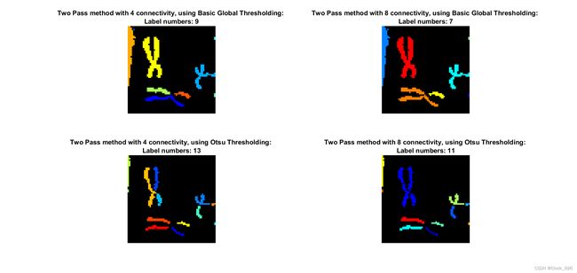
从结果上看,8连接算法在识别和标注物体方面比4连接算法更有效,某些情况下后者无法准确标注物体,并可能将单个物体识别为多个物体。8连接算法能够扫描更多的相邻像素,包括对角像素,因此能够更好地获取相邻像素信息,得到更精确的结果。不过即使是8连接算法也没有达到100% 的准确率,这表明还可以通过改进阈值法或手动调整特定像素值来进一步提高准确率。
总结来说,双通道方法与不同的连接选项和阈值技术相结合,为二值图像中的物体标注提供了一种有效的方法。根据具体应用和输入图像特征选择适当的连接和阈值方法,有助于优化对象识别过程和标注精度。
总结
对于输入图像,一共完成了以下步骤:
(1)读取并显示原始图像。对于本项目中给出的图像,每个字符都被指定了相应的像素,以成功地执行图像显示。
(2)对图像进行阈值操作并将其转换为二值图像。图像阈值处理是许多图像处理和计算机视觉应用中的关键步骤,它可以通过将灰度图像转换成二值图像,将感兴趣的对象从背景中分离出来。
(3)确定物体的1像素薄图像。图像细化是一种重要的图像处理技术,通过将物体的宽度减小到单个像素的厚度来简化二进制图像。在本例中采用Zhang-Suen算法来处理由上一步经两种阈值处理技术生成的二值图像。对于细化过程来说,选择合适的阈值处理方法至关重要。
(4)确定图像轮廓。提取二值图像中物体的轮廓是物体识别、分割和形状分析等各种图像处理任务中必不可少的一步。选择合适的阈值处理方法,对于轮廓处理同样重要。
(5)给图像中不同的物体赋予标签,连接方法采用4连接和8连接。连通分量标记(Connected Component Labeling,CCL)是图像处理和计算机视觉领域的一项重要技术,用于从二进制图像中提取不同的物体或区域。根据具体应用和输入图像特征选择适当的连接和阈值方法,有助于优化对象识别过程和标注精度。