扩散模型:DDPM代码的学习(基于minist数据集)
文章目录
- 序言
- 一参考资料
-
- ①代码来源
- ②相关概念理解
- ③公式推导及训练流程讲解
- ④搜索问题的网站
- ⑤模型运行的环境
- 二代码解读
-
- ①模型
- ②训练
- ③测试
- 三主要训练过程的解析
序言
本文主要对一个基于minist数据集搭建的DDPM模型代码中各个模块的含义进行解析,初步记录了自己了解扩散模型的一个过程,为后续的进一步学习打基础。文中的错误之处还望大家批评指正
一参考资料
①代码来源
参考的代码来源
②相关概念理解
超详细的扩散模型(Diffusion Models)原理+代码
③公式推导及训练流程讲解
DDPM1
DDPM2
④搜索问题的网站
geekgpt
此网站可以对代码进行注释,对公式推导的流程进行解释,利用的好可以帮助我们更好的理解我们所的遇到的大部分问题
⑤模型运行的环境
本文是在google drive的colab中运行的
colab的部署过程可以参考以下内容:Colab 实用教程
二代码解读
①模型
import os
import math
from abc import abstractmethod

import numpy as np
import torch
import torch.nn as nn
import torch.nn.functional as F
from tqdm import tqdm
def timestep_embedding(timesteps, dim, max_period=10000):
    """Create sinusoidal timestep embeddings.

    Args:
        timesteps (Tensor): a 1-D Tensor of N indices, one per batch element. These may be fractional.
        dim (int): the dimension of the output.
        max_period (int, optional): controls the minimum frequency of the embeddings. Defaults to 10000.

    Returns:
        Tensor: an [N x dim] Tensor of positional embeddings.
    """
    # 计算嵌入向量的一半维度
    half = dim // 2

    # 计算频率,用来生成正弦和余弦成分
    freqs = torch.exp(
        -math.log(max_period) * torch.arange(start=0, end=half, dtype=torch.float32) / half
    ).to(device=timesteps.device)

    # 计算角度参数,用于生成正弦和余弦成分
    #进行维度的扩充,将1*step转化为step*1 然后和1*half进行矩阵运算,将数据的维度扩充到了half维度(half为偶数)
    args = timesteps[:, None].float() * freqs[None]

    # 生成正弦和余弦成分,然后连接它们以形成嵌入向量
    embedding = torch.cat([torch.cos(args), torch.sin(args)], dim=-1)

    # 如果维度是奇数,添加一个额外的零维度
    if dim % 2:
        embedding = torch.cat([embedding, torch.zeros_like(embedding[:, :1])], dim=-1)

    # 返回时间步嵌入向量
    return embedding


class TimestepBlock(nn.Module):
    """
    Any module where forward() takes timestep embeddings as a second argument.
    """

    @abstractmethod
    def forward(self, x, t):
        """
        Apply the module to `x` given `t` timestep embeddings.
        """
        pass


class TimestepEmbedSequential(nn.Sequential, TimestepBlock):
    """
    A sequential module that passes timestep embeddings to the children that support it as an extra input.
    """

    def forward(self, x, t):
        for layer in self:
            if isinstance(layer, TimestepBlock):
                x = layer(x, t)
            else:
                x = layer(x)
        return x
     # layer 是 TimestepEmbedSequential 类中的每个子模块(layer)的引用。在这个循环中,我们遍历了 TimestepEmbedSequential 类中的每个子模块,并对其进行操作。如果子模块是 TimestepBlock 的实例,则调用其 forward() 方法,并将输入数据 x 和时间步骤嵌入向量 t 传递给它;否则,我们只是将输入数据 x 传递给子模块


#参数channels指定了归一化层的通道数,而nn.GroupNorm的第一个参数32表示将输入数据的通道分成32个子组,每个子组内的特征将被独立地归一化,组归一化的主要作用是解决深度神经网络中的内部协变量偏移问题,提高模型的训练稳定性,使其更适合处理不同批量大小和高分辨率数据,同时也有助于模型的泛化能力。
def norm_layer(channels):
    return nn.GroupNorm(32, channels)


class ResidualBlock(TimestepBlock):
    def __init__(self, in_channels, out_channels, time_channels, dropout):
        super().__init__()
        self.conv1 = nn.Sequential(
            norm_layer(in_channels),
            nn.SiLU(),
            nn.Conv2d(in_channels, out_channels, kernel_size=3, padding=1)
        )

        # pojection for time step embedding
        self.time_emb = nn.Sequential(
            nn.SiLU(),
            nn.Linear(time_channels, out_channels)
        )

        self.conv2 = nn.Sequential(
            norm_layer(out_channels),
            nn.SiLU(),
            nn.Dropout(p=dropout),
            nn.Conv2d(out_channels, out_channels, kernel_size=3, padding=1)
        )

        if in_channels != out_channels:
            self.shortcut = nn.Conv2d(in_channels, out_channels, kernel_size=1)
        else:
            self.shortcut = nn.Identity()


    def forward(self, x, t):
        """
        `x` has shape `[batch_size, in_dim, height, width]`
        `t` has shape `[batch_size, time_dim]`
        """
        h = self.conv1(x)
        # Add time step embeddings
        h += self.time_emb(t)[:, :, None, None]
        h = self.conv2(h)
        return h + self.shortcut(x)


class AttentionBlock(nn.Module):
    def __init__(self, channels, num_heads=1):
        """
        Attention block with shortcut

        Args:
            channels (int): channels
            num_heads (int, optional): attention heads. Defaults to 1.
        """
        super().__init__()
        self.num_heads = num_heads
        assert channels % num_heads == 0

        self.norm = norm_layer(channels)
        self.qkv = nn.Conv2d(channels, channels * 3, kernel_size=1, bias=False)
        self.proj = nn.Conv2d(channels, channels, kernel_size=1)

    def forward(self, x):
        B, C, H, W = x.shape
        qkv = self.qkv(self.norm(x))
        #将模型的维度扩充3倍
        q, k, v = qkv.reshape(B*self.num_heads, -1, H*W).chunk(3, dim=1)
        scale = 1. / math.sqrt(math.sqrt(C // self.num_heads))
        # 计算了一个用于缩放注意力分数的标度因子(scaling factor)。这个标度因子通常用于控制注意力分数的大小,以避免过大的数值,有助于稳定训练过程
        attn = torch.einsum("bct,bcs->bts", q * scale, k * scale)
       #这一行代码执行了一个张量乘法操作,并计算了注意力分数(attention scores)
        attn = attn.softmax(dim=-1)
        #进行 softmax 归一化,以确保每个位置的分数都在 [0, 1] 范围内
        h = torch.einsum("bts,bcs->bct", attn, v)
        #torch.einsum 函数是一个强大的张量运算工具,它允许用户根据一种命名约定来指定张量的操作,以实现高效的张量操作和组合。它的基本语法是
		#result = torch.einsum("ij,jk->ik", A, B)
		#这将计算两个矩阵 A 和 B 的矩阵乘法。字符串 "ij,jk->ik" 描述了两个矩阵的操作,其中 "ij" 表示 A 的行和列,而 "jk" 表示 B 的行和列,最终得到一个矩阵
        #其中 attn 和 v 是输入张量,具有以下维度:
			#attn 的形状为 (batch_size, sequence_length, num_heads),
			#其中 batch_size 表示批处理大小,sequence_length 表示序列长度,num_heads 表示注意力头的数量。
			#v 的形状为 (batch_size, sequence_length, value_dim),其中 value_dim 表示每个注意力值的维度。
			#输出张量的形状为 (batch_size, sequence_length, value_dim),它表示了加权和的结果,其中每个元素#都是通过将 attn 中的权重应用到 v 中的相应部分来计算的。
			#这种操作通常用于多头注意力机制中,其中 attn 包含了注意力分数(或权重),v 包含了值,而输出则是根#据权重对值进行加权求和的结果。这有助于模型在自注意力机制中将不同的信息聚合到输出中。
#用于执行多头注意力操作,将注意力权重应用于值并计算加权
        h = h.reshape(B, -1, H, W)
        h = self.proj(h)
        return h + x

 # 定义一个名为Upsample的自定义神经网络模块
class Upsample(nn.Module):
    def __init__(self, channels, use_conv):
        super().__init__()

        # 初始化函数,接受两个参数:channels表示输入通道数,use_conv表示是否使用卷积层

        # 将use_conv标记存储在模块中,以便后续的操作可以根据该标记来选择不同的处理方式
        self.use_conv = use_conv

        # 如果use_conv为True,即选择使用卷积层
        if use_conv:
            # 创建一个卷积层,输入通道数和输出通道数都为channels
            # 使用3x3的卷积核(kernel_size=3),并在输入周围填充1个像素(padding=1)
            self.conv = nn.Conv2d(channels, channels, kernel_size=3, padding=1)

    # 定义模块的前向传播函数,接受输入张量x作为参数
    def forward(self, x):
        # 使用F.interpolate函数对输入张量x进行上采样
        # 上采样的尺度因子为2(scale_factor=2)(将原图像的每个维度放大2倍),采用最近邻插值方式(mode="nearest")
        x = F.interpolate(x, scale_factor=2, mode="nearest")

        # 如果use_conv为True,即选择使用卷积层
        if self.use_conv:
            # 将上采样后的张量x输入到卷积层self.conv中进行卷积操作
            x = self.conv(x)

        # 返回处理后的张量x作为模块的输出
        return x


class Downsample(nn.Module):
#上采样和下采样的初始化都是输入通道数,和是否用卷积,如果不用卷积那么就用池化层进行下采样,如果用卷积,那么就用卷积核,步长为2去达到下采样的效果
    def __init__(self, channels, use_conv):
        super().__init__()
        self.use_conv = use_conv
        if use_conv:
            self.op = nn.Conv2d(channels, channels, kernel_size=3, stride=2, padding=1)
        else:
        #利用平均池化层将数据缩小为原来的1/2
            self.op = nn.AvgPool2d(stride=2)

    def forward(self, x):
        return self.op(x)


class UNetModel(nn.Module):
    """
    The full UNet model with attention and timestep embedding
    """
    def __init__(
        self,
        in_channels=3,  # 输入通道数,默认为3(适用于RGB图像)
        model_channels=128,  # 模型通道数,默认为128
        out_channels=3,  # 输出通道数,默认为3(适用于RGB图像)
        num_res_blocks=2,  # 残差块的数量,默认为2
        attention_resolutions=(8, 16),  # 注意力分辨率的元组,默认为(8, 16)
        dropout=0,  # Dropout概率,默认为0(不使用Dropout)
        channel_mult=(1, 2, 2, 2),  # 通道倍增因子的元组,默认为(1, 2, 2, 2)
        conv_resample=True,  # 是否使用卷积重采样,默认为True
        num_heads=4  # 注意力头的数量,默认为4
    ):
        super().__init__()

        # 初始化模型的各种参数
        self.in_channels = in_channels
        self.model_channels = model_channels
        self.out_channels = out_channels
        self.num_res_blocks = num_res_blocks
        self.attention_resolutions = attention_resolutions
        self.dropout = dropout
        self.channel_mult = channel_mult
        self.conv_resample = conv_resample
        self.num_heads = num_heads

        # 时间嵌入(用于处理时间信息的嵌入)
        time_embed_dim = model_channels * 4
        self.time_embed = nn.Sequential(
            nn.Linear(model_channels, time_embed_dim),
            nn.SiLU(),
            nn.Linear(time_embed_dim, time_embed_dim),
        )

        # 下采样块
        #所有的模块都是先定义,然后通过迭代的方式往模块里面加东西
        self.down_blocks = nn.ModuleList([
            TimestepEmbedSequential(nn.Conv2d(in_channels, model_channels, kernel_size=3, padding=1))
        ])
        down_block_chans = [model_channels]  # 存储下采样块每一阶段的通道数
		ch = model_channels  # 当前通道数初始化为模型通道数 初始为128
		ds = 1  # 下采样的倍数,初始值为1
		# 遍历不同阶段的下采样块
		#channel_mult模块为(1,2,2,2),下采样块每层的块数
        for level, mult in enumerate(channel_mult):
        	#num_res_blocks为残差块的数量,表示每块需要的残差快的数量
            for _ in range(num_res_blocks):
                layers = [
                #ch为输入通道数,mult * model_channels为需要输出的维度数,time_embed_dim为时间嵌入的维度
                    ResidualBlock(ch, mult * model_channels, time_embed_dim, dropout)
                    #初始化剩余块,让我们后续能用forward函数将时间嵌入到x中
                ]
                ch = mult * model_channels
                #ds为一个值,一开始为1,然后每次乘以2,这里如果ds为8或者16时需要加上一个注意力模块
                if ds in attention_resolutions:
                    layers.append(AttentionBlock(ch, num_heads=num_heads))
                #将加入了残差快和注意力块的层加入下采样块当中
                self.down_blocks.append(TimestepEmbedSequential(*layers))
                #记录每一层采样的通道数
                down_block_chans.append(ch)
            if level != len(channel_mult) - 1:  # 最后一个阶段不使用下采样
           		#这里由于之前的ch*2 所以,下采样后又恢复到了 ch,所以,我们在下采样通道中加入的ch
                self.down_blocks.append(TimestepEmbedSequential(Downsample(ch, conv_resample)))
                down_block_chans.append(ch)
                ds *= 2
             #整个流程的格式变换,128,128,64;256,256,128;256,256;

        # 中间块
        #中间块就是一个残差块+注意力块+残差块
        self.middle_block = TimestepEmbedSequential(
            ResidualBlock(ch, ch, time_embed_dim, dropout),
            AttentionBlock(ch, num_heads=num_heads),
            ResidualBlock(ch, ch, time_embed_dim, dropout)
        )

        # 上采样块
        self.up_blocks = nn.ModuleList([])
        #反过来计算通道的情况(2,2,2,1)
        for level, mult in list(enumerate(channel_mult))[::-1]:
        	#反向时残差块的数目为3
            for i in range(num_res_blocks + 1):
                layers = [
                    ResidualBlock(
                        ch + down_block_chans.pop(),
                        model_channels * mult,
                        time_embed_dim,
                        dropout
                    )
                ]
                ch = model_channels * mult
                if ds in attention_resolutions:
                    layers.append(AttentionBlock(ch, num_heads=num_heads))
                #如果level不为0,并且,i为2时(最后一块时),进行上采样
                if level and i == num_res_blocks:
                    layers.append(Upsample(ch, conv_resample))
                    ds //= 2
                self.up_blocks.append(TimestepEmbedSequential(*layers))

        # 输出层
        #只是一个正则化,激活后的再一次不改变通道数的卷积
        self.out = nn.Sequential(
            norm_layer(ch),
            nn.SiLU(),
            nn.Conv2d(model_channels, out_channels, kernel_size=3, padding=1),
        )

    def forward(self, x, timesteps):
        """Apply the model to an input batch.

        Args:
            x (Tensor): [N x C x H x W]
            timesteps (Tensor): a 1-D batch of timesteps.

        Returns:
            Tensor: [N x C x ...]
        """
        #记录每次下采样得到结果,用于后面上采样的copy and crop
        hs = []
        # 时间步嵌入
        #利用timesteps参数,计算时间步的嵌入
        #首先用timestep_embedding,将时间序列timesteps(1*n)转化为(n*model_channels)
        #然后用time_embed将之前的n*model_channels转化为 n*time_embed_dim(也就是原来的mocel_channels*4)
        emb = self.time_embed(timestep_embedding(timesteps, self.model_channels))
        #最终得到一个时间步嵌入的矩阵

        # 下采样阶段
        h = x
        for module in self.down_blocks:
        	#每次用时间步嵌入的矩阵信息emb,更新并记录每次的h
            h = module(h, emb)
            hs.append(h)

        # 中间阶段
        h = self.middle_block(h, emb)

        # 上采样阶段
        for module in self.up_blocks:
            cat_in = torch.cat([h, hs.pop()], dim=1)
            h = module(cat_in, emb)

        return self.out(h)


#线性β,只是等距的值
def linear_beta_schedule(timesteps):
    """
    beta schedule
    """
    scale = 1000 / timesteps
    beta_start = scale * 0.0001
    beta_end = scale * 0.02
    #等距生成timesteps个数值,作为β的取值
    return torch.linspace(beta_start, beta_end, timesteps, dtype=torch.float64)


#实现了一个余弦学习率调度
#timesteps: 这是一个整数参数,指定生成渐变序列的时间步数。
#s: 这是余弦调度的一个超参数,控制余弦曲线的形状。默认值为0.008。
def cosine_beta_schedule(timesteps, s=0.008):
    """
    cosine schedule
    as proposed in https://arxiv.org/abs/2102.09672
    """
    steps = timesteps + 1
    x = torch.linspace(0, timesteps, steps, dtype=torch.float64)
    #alphas_cumprod: 这个步骤计算了一个余弦曲线的累积乘积,并且通过缩放将其限制在0到1之间。这个曲线的形状由s参数控制。
    alphas_cumprod = torch.cos(((x / timesteps) + s) / (1 + s) * math.pi * 0.5) ** 2
    alphas_cumprod = alphas_cumprod / alphas_cumprod[0]
    #betas: 计算了渐变的beta值序列,通过计算相邻时间步的alphas_cumprod之间的差异。
    betas = 1 - (alphas_cumprod[1:] / alphas_cumprod[:-1])
    #最后,将beta值序列裁剪到区间[0, 0.999]之间,以确保其在有效范围内。
    return torch.clip(betas, 0, 0.999)


class GaussianDiffusion:
    def __init__(
        self,

        timesteps=1000,          # 初始化函数,设置默认时间步数为1000
        beta_schedule='linear'   # 初始化函数,设置默认的beta调度为'linear'
    ):

 		self.timesteps = timesteps  # 存储时间步数

        # 根据选择的beta调度类型,生成beta值的序列
        if beta_schedule == 'linear':
            betas = linear_beta_schedule(timesteps)
        elif beta_schedule == 'cosine':
            betas = cosine_beta_schedule(timesteps)
        else:
            raise ValueError(f'unknown beta schedule {beta_schedule}')
        self.betas = betas  # 存储beta值序列

        # 计算alpha值(1 - beta)和alpha的累积乘积(1,2,3)变为(1,2,6)

        self.alphas = 1. - self.betas
        self.alphas_cumprod = torch.cumprod(self.alphas, axis=0)
        #F.pad(a,b,c)函数,在a向量的最前面和最后面分别添加b个c元素
        self.alphas_cumprod_prev = F.pad(self.alphas_cumprod[:-1], (1, 0), value=1.)
        #这个操作的目的通常是为了在某些计算中需要使用 self.alphas_cumprod_prev 作为一个与 self.alphas_cumprod 相关的中间变量。在这种情况下,添加一个1作为起始值可以确保计算的正确性。

        # calculations for diffusion q(x_t | x_{t-1}) and others
        #计算一些用于不同公式的其他变量
        self.sqrt_alphas_cumprod = torch.sqrt(self.alphas_cumprod)
        self.sqrt_one_minus_alphas_cumprod = torch.sqrt(1.0 - self.alphas_cumprod)
        self.log_one_minus_alphas_cumprod = torch.log(1.0 - self.alphas_cumprod)
        self.sqrt_recip_alphas_cumprod = torch.sqrt(1.0 / self.alphas_cumprod)
        self.sqrt_recipm1_alphas_cumprod = torch.sqrt(1.0 / self.alphas_cumprod - 1)

        # calculations for posterior q(x_{t-1} | x_t, x_0)
        self.posterior_variance = (
            self.betas * (1.0 - self.alphas_cumprod_prev) / (1.0 - self.alphas_cumprod)
        )
        # below: log calculation clipped because the posterior variance is 0 at the beginning
        # of the diffusion chain
        #用于存储后验分布的对数方差
        self.posterior_log_variance_clipped = torch.log(self.posterior_variance.clamp(min =1e-20))
		#后验均值的系数1
        self.posterior_mean_coef1 = (
            self.betas * torch.sqrt(self.alphas_cumprod_prev) / (1.0 - self.alphas_cumprod)
        )
        #后验均值的系数2
        self.posterior_mean_coef2 = (
            (1.0 - self.alphas_cumprod_prev)
            * torch.sqrt(self.alphas)
            / (1.0 - self.alphas_cumprod)
        )

    def _extract(self, a, t, x_shape):
    	# 辅助函数:从a中提取与时间步t对应的参数
        # get the param of given timestep t
        batch_size = t.shape[0]
        out = a.to(t.device).gather(0, t).float()
        #将输出的out的形状改为只有batch_size,其余维度都为1
        out = out.reshape(batch_size, *((1,) * (len(x_shape) - 1)))
        return out

    def q_sample(self, x_start, t, noise=None):
        # forward diffusion (using the nice property): q(x_t | x_0)
        if noise is None:
            noise = torch.randn_like(x_start)
		#获得第t步的参数数据
        sqrt_alphas_cumprod_t = self._extract(self.sqrt_alphas_cumprod, t, x_start.shape)
        sqrt_one_minus_alphas_cumprod_t = self._extract(self.sqrt_one_minus_alphas_cumprod, t, x_start.shape)
		#然后和随机产生的噪声进行按比例拟合达到加噪的效果
        return sqrt_alphas_cumprod_t * x_start + sqrt_one_minus_alphas_cumprod_t * noise

    def q_mean_variance(self, x_start, t):
        # Get the mean and variance of q(x_t | x_0).
        #x_start为需要输入的图像
        mean = self._extract(self.sqrt_alphas_cumprod, t, x_start.shape) * x_start
        variance = self._extract(1.0 - self.alphas_cumprod, t, x_start.shape)
        log_variance = self._extract(self.log_one_minus_alphas_cumprod, t, x_start.shape)
        return mean, variance, log_variance

    def q_posterior_mean_variance(self, x_start, x_t, t):
        # Compute the mean and variance of the diffusion posterior: q(x_{t-1} | x_t, x_0)
        posterior_mean = (
            self._extract(self.posterior_mean_coef1, t, x_t.shape) * x_start
            + self._extract(self.posterior_mean_coef2, t, x_t.shape) * x_t
        )
        posterior_variance = self._extract(self.posterior_variance, t, x_t.shape)
        posterior_log_variance_clipped = self._extract(self.posterior_log_variance_clipped, t, x_t.shape)
        return posterior_mean, posterior_variance, posterior_log_variance_clipped

#反向预测,对于输入的x_t反向去噪noise
    def predict_start_from_noise(self, x_t, t, noise):
        # compute x_0 from x_t and pred noise: the reverse of `q_sample`
        return (
            self._extract(self.sqrt_recip_alphas_cumprod, t, x_t.shape) * x_t -
            self._extract(self.sqrt_recipm1_alphas_cumprod, t, x_t.shape) * noise
        )
	#最终返回预测的均值,方差
    def p_mean_variance(self, model, x_t, t, clip_denoised=True):
        # compute predicted mean and variance of p(x_{t-1} | x_t)
        # predict noise using model
        #unet模块学习加入了时间t(这里的t为所有值为t的向量)信息的x_t,通过参数调整,最终变为我们的反向预测噪声
        pred_noise = model(x_t, t)
        # get the predicted x_0: different from the algorithm2 in the paper
        #从反向预测噪声和x_t预测我们的开始值(去噪)
        x_recon = self.predict_start_from_noise(x_t, t, pred_noise)
        #将 x_recon 张量中的元素限制在 -1.0 到 1.0 的范围内,任何小于 -1.0 的元素都被设置为 -1.0,任何大于 1.0 的元素都被设置为 1.0。
        if clip_denoised:
            x_recon = torch.clamp(x_recon, min=-1., max=1.)
        model_mean, posterior_variance, posterior_log_variance = self.q_posterior_mean_variance(x_recon, x_t, t)
        return model_mean, posterior_variance, posterior_log_variance

    @torch.no_grad()
    #从最后一步的随机噪声向前进行去噪采样
    def p_sample(self, model, x_t, t, clip_denoised=True):
        # denoise_step: sample x_{t-1} from x_t and pred_noise
        # predict mean and variance
        model_mean, _, model_log_variance = self.p_mean_variance(model, x_t, t, clip_denoised=clip_denoised)
        noise = torch.randn_like(x_t)
        # no noise when t == 0
        nonzero_mask = ((t != 0).float().view(-1, *([1] * (len(x_t.shape) - 1))))#判断t是否为0,是0则为0,非0则为1
        # compute x_{t-1}
        pred_img = model_mean + nonzero_mask * (0.5 * model_log_variance).exp() * noise
        return pred_img

    @torch.no_grad()
    def p_sample_loop(self, model, shape):
        # denoise: reverse diffusion
        batch_size = shape[0]
        device = next(model.parameters()).device
        # start from pure noise (for each example in the batch)
        img = torch.randn(shape, device=device)
        imgs = []
        #tqdm是python中的一个库,用于创建进度条,以可视化地显示循环的进度。它可以帮助你了解循环还需要多长时间完成,特别是在处理大数据集或长时间运行的任务时非常有用。total是定义总的步数
        #采样传入的image为随机生成的噪声,也就代表了最后的x_t时的噪声
        for i in tqdm(reversed(range(0, timesteps)), desc='sampling loop time step', total=timesteps):
        	#torch.full((batch_size,), i)创建一个值都为i的向量
            img = self.p_sample(model, img, torch.full((batch_size,), i, device=device, dtype=torch.long))
            imgs.append(img.cpu().numpy())
        return imgs

    @torch.no_grad()
    def sample(self, model, image_size, batch_size=8, channels=3):
        # sample new images
        return self.p_sample_loop(model, shape=(batch_size, channels, image_size, image_size))

    def train_losses(self, model, x_start, t):
        # compute train losses
        # generate random noise

		# 随机生成一个正态分布
        noise = torch.randn_like(x_start)
        # get x_t
        #输入的图像作为x_start,正太分布噪声采用我们自己随机生成的
        #通过前向加噪,对输入图像加入t时刻的噪声(前向加入噪的噪声作为基准噪声)
        x_noisy = self.q_sample(x_start, t, noise=noise)
        #通过unet,对前向生成的噪声和t,生成我们的预测噪声
        predicted_noise = model(x_noisy, t)
        #损失函数就是生成的噪声和预测的噪声进行损失的计算
        loss = F.mse_loss(noise, predicted_noise)
        return loss
看看效果
from PIL import Image
import requests
import matplotlib.pyplot as plt
from torchvision import datasets, transforms

%matplotlib inline
url = 'http://images.cocodataset.org/val2017/000000039769.jpg'
image = Image.open(requests.get(url, stream=True).raw)
# image = Image.open("/data/000000039769.jpg")

image_size = 128
transform = transforms.Compose([
    transforms.Resize(image_size),
    transforms.CenterCrop(image_size),
    transforms.PILToTensor(),
    transforms.ConvertImageDtype(torch.float),
    transforms.Normalize(mean=[0.5, 0.5, 0.5], std=[0.5, 0.5, 0.5]),
])

x_start = transform(image).unsqueeze(0)

gaussian_diffusion = GaussianDiffusion(timesteps=500)

plt.figure(figsize=(16, 8))
for idx, t in enumerate([0, 50, 100, 200, 499]):
	#根据x_start和t生成从0~t加噪后的结果
    x_noisy = gaussian_diffusion.q_sample(x_start, t=torch.tensor([t]))
    #squeeze(): 这是一个挤压操作,它用于去除输入张量 中维度为1的维度,以简化张量的形状
    #permute(1, 2, 0): 这是一个维度置换操作,将第一个维度移到最后一个维度
    #最后对每个张量+1然后乘以127.5(原来的数为-1~1,+1变为0~2,x127.5变为0~255)
    noisy_image = (x_noisy.squeeze().permute(1, 2, 0) + 1) * 127.5
    noisy_image = noisy_image.numpy().astype(np.uint8)
    plt.subplot(1, 5, 1 + idx)
    plt.imshow(noisy_image)
    plt.axis("off")
    plt.title(f"t={t}")

②训练
准备数据集
batch_size = 64
timesteps = 500

transform = transforms.Compose([
    transforms.ToTensor(),
    transforms.Normalize(mean=[0.5], std=[0.5])
])

# use MNIST dataset
dataset = datasets.MNIST('./data', train=True, download=True, transform=transform)
train_loader = torch.utils.data.DataLoader(dataset, batch_size=batch_size, shuffle=True)
模型
# define model and diffusion
device = "cuda" if torch.cuda.is_available() else "cpu"
#这里初始化unet模块,输入输出的channel为1.注意力模块这里没有加
model = UNetModel(
    in_channels=1,
    model_channels=96,
    out_channels=1,
    channel_mult=(1, 2, 2),
    attention_resolutions=[]
)
model.to(device)
#初始化高斯扩散模型(只初始化了需要迭代的步骤为500步),时间步默认为线性生成的时间步
gaussian_diffusion = GaussianDiffusion(timesteps=timesteps)
#优化器对unet模型的参数进行优化
optimizer = torch.optim.Adam(model.parameters(), lr=5e-4)
开始训练
epochs = 10
for epoch in range(epochs):
    for step, (images, labels) in enumerate(train_loader):
        optimizer.zero_grad()

        batch_size = images.shape[0]
        images = images.to(device)

        # sample t uniformally for every example in the batch
        #随机生成batch_size个(0~timesteps)的t(对于每次训练数据,我们是随机对第其中一个t时刻的加噪过程进行训练和预测)
        t = torch.randint(0, timesteps, (batch_size,), device=device).long()
		#输入unet模型,样本图像,和t计算损失
        loss = gaussian_diffusion.train_losses(model, images, t)
        	#先随机生成一个正太分布(作为我们的加噪的正太分布)
        	#将输入的图像images作为x_start
        	#通过前向加噪,对输入的图像加入t时刻的噪声(此时生成的噪声作为我们的基准噪声)
        	#通过unet,输入上一步的基准噪声,和时间步t,我们进行对基准噪声的预测
        	#损失函数计算的就是我们的预测噪声和基准噪声之间的差距,采用的是每个像素点的均方差的计算

        if step % 200 == 0:
            print("Loss:", loss.item())
		#每次训练模型都是让我们的unet模型的参数进行优化,让我们的unet模型最终可以根据给定一个加噪了t次后的图像,和t,去生成一个对于这个基准噪声的预测。(也就是,我们的unet模型能生成和加入的噪声十分相似的噪声)
        loss.backward()
        optimizer.step()
Loss: 1.2879185676574707
Loss: 0.05010918155312538
Loss: 0.037472739815711975
Loss: 0.03259456530213356
Loss: 0.03238191455602646
Loss: 0.03526081144809723
Loss: 0.019976193085312843
Loss: 0.026588361710309982
Loss: 0.02474384568631649
Loss: 0.025454936549067497
Loss: 0.01776018552482128
Loss: 0.028406977653503418
Loss: 0.026149388402700424
Loss: 0.023932695388793945
Loss: 0.0222737155854702
Loss: 0.025710856541991234
Loss: 0.026215054094791412
Loss: 0.02046349085867405
Loss: 0.02683963067829609
Loss: 0.023800114169716835
Loss: 0.024538405239582062
Loss: 0.021686285734176636
Loss: 0.019745750352740288
Loss: 0.02584003284573555
Loss: 0.026672476902604103
Loss: 0.023941144347190857
Loss: 0.03131483495235443
Loss: 0.018094774335622787
Loss: 0.025758417323231697
Loss: 0.025309113785624504
Loss: 0.0224548801779747
Loss: 0.021184200420975685
Loss: 0.01910235919058323
Loss: 0.024598510935902596
Loss: 0.024002162739634514
Loss: 0.0232978705316782
Loss: 0.016557812690734863
Loss: 0.019946767017245293
Loss: 0.020528556779026985
Loss: 0.01813691109418869
Loss: 0.020777976140379906
Loss: 0.021010225638747215
Loss: 0.02573891542851925
Loss: 0.02588081546127796
Loss: 0.016215061768889427
Loss: 0.025008078664541245
Loss: 0.01972994953393936
Loss: 0.021410418674349785
Loss: 0.024027982726693153
Loss: 0.021927889436483383
③测试
generated_images = gaussian_diffusion.sample(model, 28, batch_size=64, channels=1)
# generated_images: [timesteps, batch_size=64, channels=1, height=28, width=28]
sampling loop time step: 100%|█████████████████████████████████████████████████████████████████████████████████████████████████████████████████████████████████████████████████████| 500/500 [00:30<00:00, 16.61it/s]
# generate new images
fig = plt.figure(figsize=(12, 12), constrained_layout=True)
#并定义了一个网格布局,该布局包含 8 行和 8 列的子图
gs = fig.add_gridspec(8, 8)

#[-1]表示生成图像的最后一个,也就是x0(最后生成的图片),将数组重新排列为8,8,28,28的形式
imgs = generated_images[-1].reshape(8, 8, 28, 28)
for n_row in range(8):
    for n_col in range(8):
    	#将图像加入8*8网格对应的位置
        f_ax = fig.add_subplot(gs[n_row, n_col])
        #将图像的值变换到0~255进行可视化
        f_ax.imshow((imgs[n_row, n_col]+1.0) * 255 / 2, cmap="gray")
        f_ax.axis("off")

可以看到我们的扩散模型生成的图像与minist数据集还是非常相似的
展示降噪的过程
# show the denoise steps
fig = plt.figure(figsize=(12, 12), constrained_layout=True)
gs = fig.add_gridspec(16, 16)

#也就是我们生成的generated_images是一个多维的矩阵,step,batchsize,28,28,1  ; 然后我们需要对第i个step过程取其中的第n_row个图片,然后去展示这个去噪的过程
for n_row in range(16):
    for n_col in range(16):
        f_ax = fig.add_subplot(gs[n_row, n_col])
        #t_idx计算为第几步的噪声,从500开始到0
        t_idx = (timesteps // 16) * n_col if n_col < 15 else -1
        #n_now为第n个图像
        img = generated_images[t_idx][n_row].reshape(28, 28)
        f_ax.imshow((img+1.0) * 255 / 2, cmap="gray")
        f_ax.axis("off")
三主要训练过程的解析


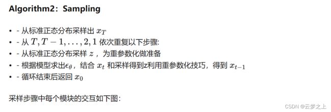

不好理解之处对于最后的sample阶段的取样过程,是如何从随机的噪声一步一步去噪恢复原图像的:
流程上讲:
如上图所示,每次第t时刻,我们首先将t时刻的噪声xt和t时刻位置的正弦编码输入unet网络,得到我们预测的噪声,然后经过对预测的噪声进行处理得到我们预测的均值和方差,然后通过参数重参化技巧,构建我们生成的预测去噪图像(这里我们每次得到的预测结果,是作为下一次新的t-1时刻的噪声xt-1),然后通过连续的迭代,最终生成初始x0时刻的图像(也就是我们最终的反向去噪图像)。
难点在于:
对于均值和方差的预测,以及预测图像的重构等过程的数学推导,可以先有个大概的印象,后续在慢慢攻克