pytorch一小时速成

目录

1.TENSORS（张量）

1.1初始化一个张量：

1.2张量的属性

1.3张量的操作

1.4 与Numpy的转换

2.数据集与数据加载

2.1加载数据集

2.2迭代和可视化数据集

 2.3创建一个自定义数据集

2.4使用DataLoaders准备数据

2.5遍历DataLoader

3数据转换

3.1TRANSFORMS

3.2ToTensor()

3.3Lambda Transforms

4建立模型

4.1建立神经网络

4.2选择训练设备

4.3定义类

4.4模型层

4.5模型参数

5 用Torch.autograd进行自动区分

5.1张量、函数和计算图

5.2梯度计算

5.3禁用梯度跟踪

5.4关于计算图的更多信息

5.5选读：张量梯度和雅各布乘积

6.优化模型参数

6.1代码

6.2超参

6.3优化循环

6.4损失函数

6.5Optimizer

6.6Full Implementation

7保存和加载模型：

7.1保存和加载模型权重

7.2保存和加载形状的模型

---

1.TENSORS（张量）

张量与NumPy的ndarrays类似，只是张量可以在GPU或其他硬件加速器上运行。事实上，张量和NumPy数组通常可以共享相同的底层内存，不需要复制数据（见与NumPy的转换）。张量还为自动分化进行了优化（我们将在后面的Autograd部分看到更多关于这一点）。如果你熟悉ndarrays，你就会对张量API很熟悉。

导入：

import torch
import numpy as np

1.1初始化一个张量：

• 直接从数据：张量可以直接从数据中创建。数据类型是自动推断出来的。

data = [[1, 2],[3, 4]]
x_data = torch.tensor(data)

• 从numpy数组：

np_array = np.array(data)
x_np = torch.from_numpy(np_array)

• 从其它张量：新的张量保留了参数张量的属性（形状、数据类型），除非明确重写。

x_ones = torch.ones_like(x_data) # 保持原有类型
print(f"Ones Tensor: \n {x_ones} \n")

x_rand = torch.rand_like(x_data, dtype=torch.float) #重写数据类型
print(f"Random Tensor: \n {x_rand} \n")

Ones Tensor:
 tensor([[1, 1],
        [1, 1]])

Random Tensor:
 tensor([[0.2035, 0.2540],
        [0.3765, 0.7375]])

• 具有随机或恒定值：shape是一个张量的元组。在下面的函数中，它决定了输出张量的维度。

shape = (2,3,)
rand_tensor = torch.rand(shape)
ones_tensor = torch.ones(shape)
zeros_tensor = torch.zeros(shape)

print(f"Random Tensor: \n {rand_tensor} \n")
print(f"Ones Tensor: \n {ones_tensor} \n")
print(f"Zeros Tensor: \n {zeros_tensor}")

Random Tensor:
 tensor([[0.5781, 0.6603, 0.3627],
        [0.5420, 0.3776, 0.4642]])

Ones Tensor:
 tensor([[1., 1., 1.],
        [1., 1., 1.]])

Zeros Tensor:
 tensor([[0., 0., 0.],
        [0., 0., 0.]])

1.2张量的属性

• 张量属性描述了它们的形状、数据类型以及存储它们的设备。

tensor = torch.rand(3,4)

print(f"Shape of tensor: {tensor.shape}")
print(f"Datatype of tensor: {tensor.dtype}")
print(f"Device tensor is stored on: {tensor.device}")

Shape of tensor: torch.Size([3, 4])
Datatype of tensor: torch.float32
Device tensor is stored on: cpu

1.3张量的操作

这里全面介绍了100多种张量操作，包括算术、线性代数、矩阵操作（转置、索引、切片）、采样等。torch — PyTorch 2.0 documentation

默认情况下，张量是在CPU上创建的。我们需要使用.to方法明确地将张量移动到GPU上（在检查GPU的可用性之后）。请记住，在不同的设备上复制大的张量，在时间和内存上都是很昂贵的!

# 如果存在GPU，将张量存储在GPU上
if torch.cuda.is_available():
    tensor = tensor.to("cuda")

• 类似Numpy的索引和切片

tensor = torch.ones(4, 4)
print(f"First row: {tensor[0]}")#第一行
print(f"First column: {tensor[:, 0]}")#第一列
print(f"Last column: {tensor[..., -1]}")#最后一列
tensor[:,1] = 0#将第二列赋值为2
print(tensor)

First row: tensor([1., 1., 1., 1.])
First column: tensor([1., 1., 1., 1.])
Last column: tensor([1., 1., 1., 1.])
tensor([[1., 0., 1., 1.],
        [1., 0., 1., 1.],
        [1., 0., 1., 1.],
        [1., 0., 1., 1.]])

• 连接张量： 你可以使用torch.cat沿着给定的维度连接一连串的张量。参见torch.stack，这是另一个与torch.cat有细微差别的张量连接选项。

t1 = torch.cat([tensor, tensor, tensor], dim=1)
print(t1)

tensor([[1., 0., 1., 1., 1., 0., 1., 1., 1., 0., 1., 1.],
        [1., 0., 1., 1., 1., 0., 1., 1., 1., 0., 1., 1.],
        [1., 0., 1., 1., 1., 0., 1., 1., 1., 0., 1., 1.],
        [1., 0., 1., 1., 1., 0., 1., 1., 1., 0., 1., 1.]])

• 算数运算，也可学习 torch.Tensor的4种乘法_torch tensor 相乘_da_kao_la的博客-CSDN博客

# 这将计算两个张量之间的矩阵乘法。 y1, y2, y3将有相同的值
# ``tensor.T`` 返回一个转置向量
y1 = tensor @ tensor.T
y2 = tensor.matmul(tensor.T)

y3 = torch.rand_like(y1)
torch.matmul(tensor, tensor.T, out=y3)


# 这将计算出元素相乘的结果。 z1, z2, z3将有相同的值
z1 = tensor * tensor
z2 = tensor.mul(tensor)

z3 = torch.rand_like(tensor)
torch.mul(tensor, tensor, out=z3)

tensor([[1., 0., 1., 1.],
        [1., 0., 1., 1.],
        [1., 0., 1., 1.],
        [1., 0., 1., 1.]])

• 单元素张量：如果有一个单元素张量，例如通过将一个张量的所有值聚集成一个值，你可以使用 item() 将其转换为一个 Python 数值：

agg = tensor.sum()
agg_item = agg.item()
print(agg_item, type(agg_item))

12.0 

• 原地操作：将结果存储到操作数中的操作被称为原地操作。它们用后缀_来表示。例如：x.copy_(y), x.t_(), 将改变x。

print(f"{tensor} \n")
tensor.add_(5)
print(tensor)

tensor([[1., 0., 1., 1.],
        [1., 0., 1., 1.],
        [1., 0., 1., 1.],
        [1., 0., 1., 1.]])

tensor([[6., 5., 6., 6.],
        [6., 5., 6., 6.],
        [6., 5., 6., 6.],
        [6., 5., 6., 6.]])

1.4 与Numpy的转换

• Tensor 转为 NumPy array

t = torch.ones(5)
print(f"t: {t}")
n = t.numpy()
print(f"n: {n}")

t: tensor([1., 1., 1., 1., 1.])
n: [1. 1. 1. 1. 1.]

t.add_(1)
print(f"t: {t}")
print(f"n: {n}")

t: tensor([2., 2., 2., 2., 2.])
n: [2. 2. 2. 2. 2.]

• NumPy 转为 Tensor

n = np.ones(5)
t = torch.from_numpy(n)

np.add(n, 1, out=n)
print(f"t: {t}")
print(f"n: {n}")

t: tensor([2., 2., 2., 2., 2.], dtype=torch.float64)
n: [2. 2. 2. 2. 2.]

2.数据集与数据加载

处理数据样本的代码可能会变得杂乱无章且难以维护；希望我们的数据集代码能够与我们的模型训练代码解耦，以提高可读性和模块化程度。PyTorch提供了两个数据基元：torch.utils.data.DataLoader和torch.utils.data.Dataset，允许你使用预先加载的数据集以及你自己的数据。Dataset存储了样本及其相应的标签，而DataLoader则围绕Dataset包装了一个可迭代的数据集，以便能够方便地访问这些样本。

PyTorch领域库提供了一些预加载的数据集（如FashionMNIST），这些数据集子类为torch.utils.data.Dataset，并实现了针对特定数据的功能。它们可以用来为你的模型建立原型和基准。你可以在这里找到它们：图像数据集、文本数据集和音频数据集

2.1加载数据集

下面是一个如何从TorchVision加载Fashion-MNIST数据集的例子。Fashion-MNIST是一个由60,000个训练实例和10,000个测试实例组成的Zalando的文章图像数据集。每个例子包括一个28×28的灰度图像和10个类别中的一个相关标签。 

 详细学习：torch.utils.data — PyTorch 2.0 documentation

我们用以下参数加载FashionMNIST数据集：

1. root是存储训练/测试数据的路径、
2. train指的是训练或测试数据集、
3. download=True如果根目录下没有数据，则从互联网上下载数据。
4. transform和target_transform指定特征和标签的转换。

import torch
from torch.utils.data import Dataset
from torchvision import datasets
from torchvision.transforms import ToTensor
import matplotlib.pyplot as plt


training_data = datasets.FashionMNIST(
    root="data",
    train=True,
    download=True,
    transform=ToTensor()
)

test_data = datasets.FashionMNIST(
    root="data",
    train=False,
    download=True,
    transform=ToTensor()
)




out:
Downloading http://fashion-mnist.s3-website.eu-central-1.amazonaws.com/train-images-idx3-ubyte.gz
Downloading http://fashion-mnist.s3-website.eu-central-1.amazonaws.com/train-images-idx3-ubyte.gz to data/FashionMNIST/raw/train-images-idx3-ubyte.gz

  0%|          | 0/26421880 [00:00

2.2迭代和可视化数据集

我们可以像列表一样手动索引数据集：training_data[index]。我们使用matplotlib来可视化训练数据中的一些样本。

labels_map = {
    0: "T-Shirt",
    1: "Trouser",
    2: "Pullover",
    3: "Dress",
    4: "Coat",
    5: "Sandal",
    6: "Shirt",
    7: "Sneaker",
    8: "Bag",
    9: "Ankle Boot",
}
figure = plt.figure(figsize=(8, 8))
cols, rows = 3, 3
for i in range(1, cols * rows + 1):
#在0-len(training_data)之间随机生成1行，或一个
    sample_idx = torch.randint(len(training_data), size=(1,)).item()
#.item()用于在只包含一个元素的tensor中提取值，注意是只包含一个元素，否则的话使用.tolist()
    img, label = training_data[sample_idx]
    figure.add_subplot(rows, cols, i)
"""
add_subplot(rows,cols,loc,sharex,sharey)
cows: 行数
cols ： 列数
loc ： 位置 （位置计数在画布中从左到右，从上到下，如下2,2画布中）
sharex: 所有子图共用一条x轴
sharey：所有子图共用一条y轴
"""
    plt.title(labels_map[label])
    plt.axis("off")##不显示坐标轴及坐标轴标签
    plt.imshow(img.squeeze(), cmap="gray")
plt.show()

 2.3创建一个自定义数据集

一个自定义的数据集类必须实现三个函数：__init__, __len__, 和 __getitem__。看看这个实现；FashionMNIST的图像被存储在一个目录img_dir中，它们的标签被分别存储在一个CSV文件annotations_file中。

# 导入必要的库
import os # 用于处理文件和目录路径
import pandas as pd # 用于读取csv文件
from torchvision.io import read_image # 用于读取图像数据

# 定义一个自定义数据集的类，继承自torch.utils.data.Dataset
class CustomImageDataset(Dataset):
    def __init__(self, annotations_file, img_dir, transform=None, target_transform=None):
        # 读取包含图像文件名和标签的csv文件，并存储在img_labels变量中
        self.img_labels = pd.read_csv(annotations_file)
        # 存储图像所在的目录路径
        self.img_dir = img_dir
        # 保存数据集的图像变换和标签变换方法
        self.transform = transform
        self.target_transform = target_transform

    def __len__(self):
        # 返回数据集中图像的数量
        return len(self.img_labels)

    def __getitem__(self, idx):
        # 拼接图像文件的完整路径
        img_path = os.path.join(self.img_dir, self.img_labels.iloc[idx, 0])
        # 读取图像数据
        image = read_image(img_path)
        # 读取图像对应的标签
        label = self.img_labels.iloc[idx, 1]
        # 对图像进行变换
        if self.transform:
            image = self.transform(image)
        # 对标签进行变换
        if self.target_transform:
            label = self.target_transform(label)
        # 返回变换后的图像和标签
        return image, label

• __init__：在实例化数据集对象时，__init__函数会运行一次。我们初始化包含图像的目录、注释文件和两种转换（在下一节有更详细的介绍）。label.csv文件：

tshirt1.jpg, 0
tshirt2.jpg, 0
......
ankleboot999.jpg, 9

def __init__(self, annotations_file, img_dir, transform=None, target_transform=None):
    self.img_labels = pd.read_csv(annotations_file)
    self.img_dir = img_dir
    self.transform = transform
    self.target_transform = target_transform

• __len__：函数__len__返回我们数据集中的样本数。

def __len__(self):
    return len(self.img_labels)

• __getitem__：函数 __getitem__ 在给定的索引idx处加载并返回数据集中的一个样本。基于索引，它确定图像在磁盘上的位置，使用read_image将其转换为张量，从self.img_labels中的csv数据中获取相应的标签，对其调用转换函数（如果适用），并在一个元组中返回张量图像和相应标签。

def __getitem__(self, idx):
    img_path = os.path.join(self.img_dir, self.img_labels.iloc[idx, 0])
    image = read_image(img_path)
    label = self.img_labels.iloc[idx, 1]
    if self.transform:
        image = self.transform(image)
    if self.target_transform:
        label = self.target_transform(label)
    return image, label

2.4使用DataLoaders准备数据

Dataset每次都会检索我们的数据集的特征和标签。在训练模型时，我们通常希望以 "小批量 "的方式传递样本，在每个epoch中重新洗牌数据以减少模型的过拟合，并使用Python的多处理功能来加快数据的检索速度。

DataLoader是一个可迭代的，它用一个简单的API为我们抽象了这种复杂性。

from torch.utils.data import DataLoader
#shuffle是否打乱
train_dataloader = DataLoader(training_data, batch_size=64, shuffle=True)
test_dataloader = DataLoader(test_data, batch_size=64, shuffle=True)

2.5遍历DataLoader

我们已经将该数据集加载到DataLoader中，并可以根据需要对数据集进行迭代。下面的每次迭代都会返回一批train_features和train_labels（分别包含batch_size=64的特征和标签）。因为我们指定了shuffle=True，所以在我们迭代完所有的批次后，数据会被洗牌（要想对数据加载顺序进行更精细的控制，请看Samplers）。

# Display image and label.
train_features, train_labels = next(iter(train_dataloader))
print(f"Feature batch shape: {train_features.size()}")
print(f"Labels batch shape: {train_labels.size()}")
img = train_features[0].squeeze()
label = train_labels[0]
plt.imshow(img, cmap="gray")
plt.show()
print(f"Label: {label}")

out：
Feature batch shape: torch.Size([64, 1, 28, 28])
Labels batch shape: torch.Size([64])
Label: 5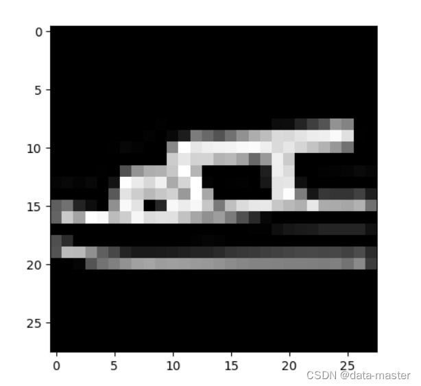

3数据转换

详细学习：Transforming and augmenting images — Torchvision 0.15 documentation

3.1TRANSFORMS

数据并不总是以训练机器学习算法所需的最终处理形式出现。我们使用转换来对数据进行一些处理，使其适合训练。

所有的TorchVision数据集都有两个参数--用于修改特征的transform和用于修改标签的target_transform--它们接受包含转换逻辑的callables。torchvision.transform模块提供了几个常用的转换。

FashionMNIST的特征是PIL图像格式的，标签是整数。对于训练，我们需要将特征作为归一化的张量，将标签作为one-hot encoded tensors。为了进行这些转换，我们使用ToTensor和Lambda。

import torch
from torchvision import datasets
from torchvision.transforms import ToTensor, Lambda

ds = datasets.FashionMNIST(
    root="data",
    train=True,
    download=True,
    transform=ToTensor(),
    target_transform=Lambda(lambda y: torch.zeros(10, dtype=torch.float).scatter_(0, torch.tensor(y), value=1))
)

3.2ToTensor()

ToTensor将PIL图像或NumPy的ndarray转换为FloatTensor，并将图像的像素强度值在[0., 1.]范围内进行缩放。Transforming and augmenting images — Torchvision 0.15 documentation

3.3Lambda Transforms

Lambda变换应用任何用户定义的Lambda函数。在这里，我们定义了一个函数，将整数变成一个one-hot encoded tensor。它首先创建一个大小为10（我们数据集中的标签数量）的零张量，并调用scatter_，在标签y给出的索引上分配一个值=1。

target_transform = Lambda(lambda y: torch.zeros(
    10, dtype=torch.float).scatter_(dim=0, index=torch.tensor(y), value=1))

4建立模型

4.1建立神经网络

神经网络由对数据进行操作的层/模块组成。torch.nn命名空间提供了您构建自己的神经网络所需的所有构件。PyTorch中的每个模块都子类化了nn.Module。一个神经网络本身就是一个由其他模块（层）组成的模块。这种嵌套结构允许轻松构建和管理复杂的架构。torch.nn — PyTorch 2.0 documentation

建立一个神经网络来对FashionMNIST数据集中的图像进行分类。

import os
import torch
from torch import nn
from torch.utils.data import DataLoader
from torchvision import datasets, transforms

4.2选择训练设备

我们希望能够在像GPU这样的硬件加速器上训练我们的模型，如果它是可用的。让我们检查一下torch.cuda是否可用，否则我们继续使用CPU。

device = "cuda" if torch.cuda.is_available() else "cpu"
print(f"Using {device} device")

out：Using cuda device

4.3定义类

我们通过子类化 nn.Module 来定义我们的神经网络，并在 __init__ 中初始化神经网络层。每个 nn.Module 子类都在 forward 方法中实现了对输入数据的操作。

class NeuralNetwork(nn.Module):
"""
在初始化方法中，首先调用父类的初始化方法，然后定义了一个flatten层，用于将输入的28*28的图像张量展平
为一维张量。接下来，使用nn.Sequential方法定义了一个包含三个线性层和两个ReLU激活函数的神经网络模
型。其中，第一个线性层的输入维度为2828，输出维度为512；第二个线性层的输入维度为512，输出维度为512；
第三个线性层的输入维度为512，输出维度为10，对应10个类别。在forward方法中，先将输入张量展平为一维张
量，然后将其输入到神经网络中进行前向传播，最后返回输出张量，即每个类别的得分（logits）。
"""
    def __init__(self):
        super().__init__()  # 继承父类的初始化方法
        self.flatten = nn.Flatten()  # 将输入张量展平为一维张量
        self.linear_relu_stack = nn.Sequential(
            nn.Linear(28*28, 512),  # 第一个隐含层，包含512个神经元
            nn.ReLU(),  # 使用ReLU激活函数
            nn.Linear(512, 512),  # 第二个隐含层，包含512个神经元
            nn.ReLU(),  # 使用ReLU激活函数
            nn.Linear(512, 10),  # 输出层，包含10个神经元，对应10个类别
        )

    def forward(self, x):
        x = self.flatten(x)  # 将输入张量展平为一维张量
        logits = self.linear_relu_stack(x)  # 输入到神经网络中进行前向传播
        return logits  # 返回输出张量，即每个类别的得分（logits）

model = NeuralNetwork().to(device)
print(model)

NeuralNetwork(
  (flatten): Flatten(start_dim=1, end_dim=-1)
  (linear_relu_stack): Sequential(
    (0): Linear(in_features=784, out_features=512, bias=True)
    (1): ReLU()
    (2): Linear(in_features=512, out_features=512, bias=True)
    (3): ReLU()
    (4): Linear(in_features=512, out_features=10, bias=True)
  )
)

注意：为了使用这个模型，我们把输入数据传给它。这就执行了模型的转发，以及一些后台操作。不要直接调用model.forward()!

在输入上调用模型会返回一个二维张量，其中dim=0对应于每个类的10个原始预测值的输出，dim=1对应于每个输出的单独值。我们通过nn.Softmax模块的一个实例来获得预测概率。

X = torch.rand(1, 28, 28, device=device)  # 创建一个大小为[1,28,28]的张量X，
#表示一张28*28的图像
logits = model(X)  # 使用神经网络模型model对X进行预测，得到一个大小为[1,10]的张量logits
pred_probab = nn.Softmax(dim=1)(logits)  # 对logits进行softmax操作，得到一个大小为[1,10]的张量
#pred_probab，其中每个元素表示对应类别的概率值
y_pred = pred_probab.argmax(1)  # 找到pred_probab中每行概率值最大的类别索引，得到一个大小为[1]
#的张量y_pred
print(f"Predicted class: {y_pred}")  # 输出预测结果

其中，X是一个大小为[1,28,28]的张量，表示一张28*28像素的图像。logits是神经网络模型对输入图像X的预测结果，它是一个大小为[1,10]的张量，其中每个元素表示对应类别的得分（logits）。pred_probab是对logits进行softmax操作后得到的概率值，它也是一个大小为[1,10]的张量，其中每个元素表示对应类别的概率值。y_pred是根据概率值得到的预测结果，它是一个大小为[1]的张量，其中的元素为对应类别的索引值。最后，通过print函数输出预测结果。

其中，nn.Softmax(dim=1)表示对logits张量的每一行进行softmax操作，得到一个大小为[1,10]的概率值张量。argmax(1)表示沿着第一维求最大值的索引值，即得到每一行概率值最大的类别索引。

4.4模型层

让我们分解一下FashionMNIST模型中的各层。为了说明这一点，我们将采取一个由3张大小为28x28的图像组成的样本minibatch ，看看当我们把它通过网络时发生了什么。

input_image = torch.rand(3,28,28)
print(input_image.size())

torch.Size([3, 28, 28])

• nn.Flatten

我们初始化nn.Flatten层，将每个28x28的二维图像转换为784个像素值的连续数组（minibatch的维度（dim=0）被保持）。Flatten — PyTorch 2.0 documentation

flatten = nn.Flatten()
flat_image = flatten(input_image)
print(flat_image.size())

torch.Size([3, 784])

• nn.Linear

线性层是一个模块，使用其存储的权重和偏置对输入进行线性转换。Linear — PyTorch 2.0 documentation

layer1 = nn.Linear(in_features=28*28, out_features=20)  # 定义一个线性变换，
#将28*28个输入特征转换为20个输出特征
hidden1 = layer1(flat_image)  # 对输入图像进行线性变换，得到第一层隐藏层的
#输出hidden1
print(hidden1.size())  # 输出hidden1的大小

• nn.ReLU

非线性激活是在模型的输入和输出之间建立复杂的映射关系。它们被应用于线性转换之后，以引入非线性，帮助神经网络学习各种各样的现象。在这个模型中，我们在线性层之间使用了nn.ReLU，但还有其他激活方式可以在你的模型中引入非线性。ReLU — PyTorch 2.0 documentation

print(f"Before ReLU: {hidden1}\n\n")
hidden1 = nn.ReLU()(hidden1)
print(f"After ReLU: {hidden1}")

Before ReLU: tensor([[ 0.1508, -0.1361,  0.4645,  0.0927, -0.2299, -0.1817,  0.2677, -0.0446,
          0.3549, -0.6060,  0.6264, -0.1267, -0.4965,  0.1950, -0.1949,  0.1069,
         -0.1537,  0.0917,  0.2399, -0.2090],
        [ 0.3523,  0.1335,  0.4606,  0.0206, -0.1106, -0.1060, -0.0374,  0.0810,
          0.1447, -0.5355,  0.3697,  0.1383, -0.0173,  0.0873, -0.4043,  0.2586,
         -0.0361, -0.2410,  0.1007, -0.2023],
        [ 0.0824,  0.4504,  0.5396, -0.0575, -0.1640, -0.2814,  0.0825,  0.2368,
         -0.0282, -0.7432,  0.2132, -0.0103, -0.2574, -0.3539, -0.5158,  0.0916,
         -0.1453,  0.0370,  0.2656, -0.4123]], grad_fn=)


After ReLU: tensor([[0.1508, 0.0000, 0.4645, 0.0927, 0.0000, 0.0000, 0.2677, 0.0000, 0.3549,
         0.0000, 0.6264, 0.0000, 0.0000, 0.1950, 0.0000, 0.1069, 0.0000, 0.0917,
         0.2399, 0.0000],
        [0.3523, 0.1335, 0.4606, 0.0206, 0.0000, 0.0000, 0.0000, 0.0810, 0.1447,
         0.0000, 0.3697, 0.1383, 0.0000, 0.0873, 0.0000, 0.2586, 0.0000, 0.0000,
         0.1007, 0.0000],
        [0.0824, 0.4504, 0.5396, 0.0000, 0.0000, 0.0000, 0.0825, 0.2368, 0.0000,
         0.0000, 0.2132, 0.0000, 0.0000, 0.0000, 0.0000, 0.0916, 0.0000, 0.0370,
         0.2656, 0.0000]], grad_fn=)

• nn.Sequential

nn.Sequential是一个模块的有序容器。数据以定义的相同顺序通过所有的模块。你可以使用顺序容器把一个快速的网络放在一起，比如seq_modules。Sequential — PyTorch 2.0 documentation

seq_modules = nn.Sequential(
    flatten,
    layer1,
    nn.ReLU(),
    nn.Linear(20, 10)
)
input_image = torch.rand(3,28,28)
logits = seq_modules(input_image)

• nn.Softmax

神经网络的最后一个线性层返回对数--[-infty, infty]中的原始值--并传递给nn.Softmax模块。对数被缩放为数值[0, 1]，代表模型对每个类别的预测概率。 dim参数表示数值必须和为1的维度。

softmax = nn.Softmax(dim=1)
pred_probab = softmax(logits)

4.5模型参数

神经网络中的许多层都是参数化的，即有相关的权重和偏置，在训练中被优化。子类化 nn.Module 会自动跟踪你的模型对象中定义的所有字段，并使用你的模型的 parameters() 或named_parameters() 方法访问所有参数。

在这个例子中，我们遍历每个参数，并打印其大小和预览其数值。

print(f"Model structure: {model}\n\n")

for name, param in model.named_parameters():
    print(f"Layer: {name} | Size: {param.size()} | Values : {param[:2]} \n")

out：
Model structure: NeuralNetwork(
  (flatten): Flatten(start_dim=1, end_dim=-1)
  (linear_relu_stack): Sequential(
    (0): Linear(in_features=784, out_features=512, bias=True)
    (1): ReLU()
    (2): Linear(in_features=512, out_features=512, bias=True)
    (3): ReLU()
    (4): Linear(in_features=512, out_features=10, bias=True)
  )
)


Layer: linear_relu_stack.0.weight | Size: torch.Size([512, 784]) | Values : tensor([[ 0.0014, -0.0149, -0.0116,  ..., -0.0138,  0.0064, -0.0345],
        [-0.0096, -0.0125,  0.0242,  ..., -0.0279,  0.0179, -0.0087]],
       device='cuda:0', grad_fn=)

Layer: linear_relu_stack.0.bias | Size: torch.Size([512]) | Values : tensor([-0.0213,  0.0056], device='cuda:0', grad_fn=)

Layer: linear_relu_stack.2.weight | Size: torch.Size([512, 512]) | Values : tensor([[-0.0031,  0.0060,  0.0231,  ...,  0.0035,  0.0018, -0.0191],
        [ 0.0176,  0.0423,  0.0151,  ...,  0.0151, -0.0368,  0.0293]],
       device='cuda:0', grad_fn=)

Layer: linear_relu_stack.2.bias | Size: torch.Size([512]) | Values : tensor([-0.0222, -0.0252], device='cuda:0', grad_fn=)

Layer: linear_relu_stack.4.weight | Size: torch.Size([10, 512]) | Values : tensor([[ 0.0440,  0.0164,  0.0411,  ...,  0.0256,  0.0181,  0.0258],
        [-0.0368,  0.0083,  0.0180,  ...,  0.0178,  0.0016,  0.0072]],
       device='cuda:0', grad_fn=)

Layer: linear_relu_stack.4.bias | Size: torch.Size([10]) | Values : tensor([-0.0075,  0.0186], device='cuda:0', grad_fn=)

5 用Torch.autograd进行自动区分

在训练神经网络时，最常使用的算法是反向传播法。在这种算法中，参数（模型权重）根据损失函数相对于给定参数的梯度来调整。Autograd mechanics — PyTorch 2.0 documentation

为了计算这些梯度，PyTorch有一个内置的微分引擎，叫做torch.autograd。它支持对任何计算图的梯度进行自动计算。

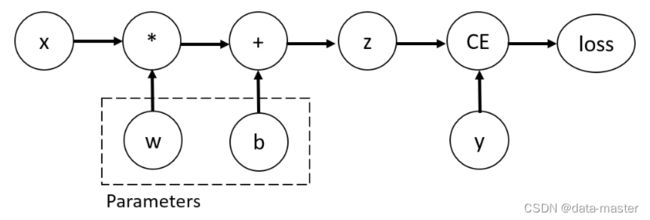
考虑最简单的单层神经网络，输入x，参数w和b，以及一些损失函数。它可以在PyTorch中以如下方式定义：

import torch

x = torch.ones(5)  # input tensor
y = torch.zeros(3)  # expected output
w = torch.randn(5, 3, requires_grad=True)
b = torch.randn(3, requires_grad=True)
z = torch.matmul(x, w)+b
loss = torch.nn.functional.binary_cross_entropy_with_logits(z, y)

5.1张量、函数和计算图

在这个网络中，w和b是参数，我们需要进行优化。因此，我们需要能够计算损失函数相对于这些变量的梯度。为了做到这一点，我们设置了这些张量的 requires_grad 属性。

注意事项：你可以在创建张量时设置requires_grad的值，或者在以后使用x.requires_grad_(True)方法。

 我们应用于张量来构建计算图的函数实际上是一个函数类的对象。这个对象知道如何在前进方向上计算函数，也知道如何在后向传播步骤中计算其导数。对后向传播函数的引用被存储在张量的grad_fn属性中。你可以在文档中找到更多关于Function的信息。

print(f"Gradient function for z = {z.grad_fn}")
print(f"Gradient function for loss = {loss.grad_fn}")

out：
Gradient function for z = 
Gradient function for loss = 

5.2梯度计算

为了优化神经网络中的参数权重，我们需要计算损失函数相对于参数的导数、和在固定的x和y值。为了计算这些导数，我们调用loss.backward()，然后从w.grad和b.grad中检索出数值：

loss.backward()
print(w.grad)
print(b.grad)

out：
tensor([[0.0784, 0.0464, 0.0931],
        [0.0784, 0.0464, 0.0931],
        [0.0784, 0.0464, 0.0931],
        [0.0784, 0.0464, 0.0931],
        [0.0784, 0.0464, 0.0931]])
tensor([0.0784, 0.0464, 0.0931])

注意事项：

我们只能获得计算图的叶子节点的梯度属性，这些节点的requires_grad属性设置为True。对于我们图中的所有其他节点，梯度将不可用。

出于性能方面的考虑，我们只能在一个给定的图上使用后向计算一次来进行梯度计算。如果我们需要在同一个图上进行多次后向调用，我们需要在后向调用中传递 retain_graph=True。

5.3禁用梯度跟踪

默认情况下，所有带有require_grad=True的张量都在跟踪它们的计算历史并支持梯度计算。然而，在某些情况下，我们不需要这样做，例如，当我们已经训练了模型，只是想把它应用于一些输入数据，也就是说，我们只想通过网络进行前向计算。我们可以通过用torch.no_grad()块包围我们的计算代码来停止跟踪计算：

z = torch.matmul(x, w)+b
print(z.requires_grad)

with torch.no_grad():
    z = torch.matmul(x, w)+b
print(z.requires_grad)

True
False

另一种实现相同结果的方法是在张量上使用detach()方法：

z = torch.matmul(x, w)+b
z_det = z.detach()
print(z_det.requires_grad)

False

你可能想禁用梯度跟踪，有一些原因：
将你的神经网络中的一些参数标记为冻结参数。

当你只做前向传递时，为了加快计算速度，因为对不跟踪梯度的张量的计算会更有效率。

5.4关于计算图的更多信息

从概念上讲，autograd在一个由Function对象组成的有向无环图（DAG）中保存了数据（张量）和所有执行的操作（以及产生的新张量）的记录。在这个DAG中，叶子是输入张量，根部是输出张量。通过追踪这个图从根到叶，你可以使用链式规则自动计算梯度。

在一个正向传递中，autograd同时做两件事：

1. 运行所请求的操作，计算出一个结果张量

2. 在DAG中保持该操作的梯度函数。

当在DAG根部调用.backward()时，后向传递就会启动：

1. 计算每个.grad_fn的梯度、
2. 将它们累积到各个张量的.grad属性中。
3. 使用连锁规则，一直传播到叶子张量。

注意事项：

在PyTorch中，DAG是动态的。需要注意的是，图是从头开始重新创建的；在每次调用.backward()后，autograd开始填充一个新的图。这正是允许你在模型中使用控制流语句的原因；如果需要，你可以在每次迭代时改变形状、大小和操作。

5.5选读：张量梯度和雅各布乘积

在许多情况下，我们有一个标量损失函数，我们需要计算相对于某些参数的梯度。然而，有些情况下，输出函数是一个任意的张量。在这种情况下，PyTorch允许你计算所谓的雅各布乘积，而不是实际的梯度。

inp = torch.eye(4, 5, requires_grad=True)
out = (inp+1).pow(2).t()
out.backward(torch.ones_like(out), retain_graph=True)
print(f"First call\n{inp.grad}")
out.backward(torch.ones_like(out), retain_graph=True)
print(f"\nSecond call\n{inp.grad}")
inp.grad.zero_()
out.backward(torch.ones_like(out), retain_graph=True)
print(f"\nCall after zeroing gradients\n{inp.grad}")

First call
tensor([[4., 2., 2., 2., 2.],
        [2., 4., 2., 2., 2.],
        [2., 2., 4., 2., 2.],
        [2., 2., 2., 4., 2.]])

Second call
tensor([[8., 4., 4., 4., 4.],
        [4., 8., 4., 4., 4.],
        [4., 4., 8., 4., 4.],
        [4., 4., 4., 8., 4.]])

Call after zeroing gradients
tensor([[4., 2., 2., 2., 2.],
        [2., 4., 2., 2., 2.],
        [2., 2., 4., 2., 2.],
        [2., 2., 2., 4., 2.]])

6.优化模型参数

现在，我们有了一个模型和数据，是时候通过在数据上优化模型的参数来训练、验证和测试我们的模型了。训练模型是一个迭代的过程；在每次迭代中，模型对输出进行预测，计算其预测的误差（损失），收集误差相对于其参数的导数（正如我们在上一节看到的），并使用梯度下降优化这些参数。

6.1代码

我们从前面关于数据集和数据加载器以及建立模型的章节中加载代码。

# 导入 PyTorch 相关模块
import torch
from torch import nn
from torch.utils.data import DataLoader
from torchvision import datasets
from torchvision.transforms import ToTensor

# 下载并准备 FashionMNIST 数据集
training_data = datasets.FashionMNIST(
    root="data",              # 数据集保存路径
    train=True,               # 加载训练集
    download=True,            # 如果本地没有数据集，则从互联网下载
    transform=ToTensor()      # 将图像转换为张量
)

test_data = datasets.FashionMNIST(
    root="data",              # 数据集保存路径
    train=False,              # 加载测试集
    download=True,            # 如果本地没有数据集，则从互联网下载
    transform=ToTensor()      # 将图像转换为张量
)

# 创建训练和测试数据的 DataLoader
train_dataloader = DataLoader(training_data, batch_size=64)
test_dataloader = DataLoader(test_data, batch_size=64)

# 定义神经网络模型
class NeuralNetwork(nn.Module):
    def __init__(self):
        super(NeuralNetwork, self).__init__()
        self.flatten = nn.Flatten()  # 将图像张量展平为向量
        self.linear_relu_stack = nn.Sequential(  # 定义全连接层
            nn.Linear(28*28, 512),   # 第一层输入大小为 28*28，输出大小为 512
            nn.ReLU(),               # 激活函数
            nn.Linear(512, 512),     # 第二层输入和输出大小均为 512
            nn.ReLU(),               # 激活函数
            nn.Linear(512, 10),      # 最后一层输入为 512，输出为 10（10 个类别）
        )

    def forward(self, x):
        x = self.flatten(x)                 # 展平图像张量
        logits = self.linear_relu_stack(x)  # 应用全连接层
        return logits

# 创建神经网络实例
model = NeuralNetwork()

6.2超参

超参数是可调整的参数，让你控制模型优化过程。不同的超参数值会影响模型的训练和收敛率（阅读更多关于超参数调整的内容）

我们为训练定义了以下超参数：

1. Number of Epochs - 迭代数据集的次数

2. Batch Size - 在更新参数之前通过网络传播的数据样本数量

3. 学习率--在每个批次/纪元更新模型参数的数量。较小的值产生缓慢的学习速度，而较大的值可能导致训练期间的不可预测的行为。

learning_rate = 1e-3
batch_size = 64
epochs = 5

6.3优化循环

一旦我们设定了超参数，我们就可以通过优化循环来训练和优化我们的模型。优化循环的每一次迭代都被称为一个 epoch。

每个epoch由两个主要部分组成：

1. 训练循环 - 迭代训练数据集并试图收敛到最佳参数。
2. 验证/测试循环--迭代测试数据集，检查模型性能是否在提高。

6.4损失函数

当遇到一些训练数据时，我们未经训练的网络很可能不会给出正确的答案。损失函数衡量的是获得的结果与目标值的不相似程度，它是我们在训练期间想要最小化的损失函数。为了计算损失，我们使用给定数据样本的输入进行预测，并与真实数据标签值进行比较。torch.nn — PyTorch 2.0 documentation

torch.optim — PyTorch 2.0 documentation

Warmstarting model using parameters from a different model in PyTorch — PyTorch Tutorials 2.0.0+cu117 documentation

常见的损失函数包括用于回归任务的 nn.MSELoss（均方误差）和用于分类的 nn.NLLLoss（负对数似然）。

我们将模型的输出对数传递给nn.CrossEntropyLoss，它将对对数进行归一化处理并计算预测误差。

# Initialize the loss function
loss_fn = nn.CrossEntropyLoss()

6.5Optimizer

优化是调整模型参数以减少每个训练步骤中的模型误差的过程。优化算法定义了这个过程是如何进行的（在这个例子中，我们使用随机梯度下降法）。所有的优化逻辑都被封装在优化器对象中。在这里，我们使用SGD优化器；此外，PyTorch中还有许多不同的优化器，如ADAM和RMSProp，它们对不同类型的模型和数据有更好的效果。

我们通过注册需要训练的模型参数来初始化优化器，并传入学习率超参数。

optimizer = torch.optim.SGD(model.parameters(), lr=learning_rate)

1. 调用optimizer.zero_grad()来重置模型参数的梯度。梯度默认为累加；为了防止重复计算，我们在每次迭代时明确地将其归零。

2. 通过调用loss.backward()对预测损失进行反向传播。PyTorch将损失的梯度与每个参数联系在一起。

3. 一旦我们有了梯度，我们就可以调用optimizer.step()，通过后向传递中收集的梯度来调整参数。

6.6Full Implementation

我们定义了train_loop和test_loop，train_loop负责循环我们的优化代码，test_loop负责根据测试数据评估模型的性能。

def train_loop(dataloader, model, loss_fn, optimizer):
    size = len(dataloader.dataset)  # 获取数据集的大小
    for batch, (X, y) in enumerate(dataloader):  # 遍历数据集
        # Compute prediction and loss
        pred = model(X)  # 模型预测
        loss = loss_fn(pred, y)  # 计算损失

        # Backpropagation
        optimizer.zero_grad()  # 梯度清零
        loss.backward()  # 反向传播
        optimizer.step()  # 更新模型参数

        if batch % 100 == 0:  # 每100个batch打印一次损失
            loss, current = loss.item(), (batch + 1) * len(X)
            print(f"loss: {loss:>7f}  [{current:>5d}/{size:>5d}]")  # 打印损失


def test_loop(dataloader, model, loss_fn):
    size = len(dataloader.dataset)  # 获取数据集的大小
    num_batches = len(dataloader)  # 获取数据集batch的个数
    test_loss, correct = 0, 0

    with torch.no_grad():  # 不需要计算梯度
        for X, y in dataloader:  # 遍历数据集
            X, y = X.to(device), y.to(device)#转换为张量
            pred = model(X)  # 模型预测
            test_loss += loss_fn(pred, y).item()  # 计算损失
            correct += (pred.argmax(1) == y).type(torch.float).sum().item()  # 计算正确率

    test_loss /= num_batches  # 计算平均损失
    correct /= size  # 计算正确率
    print(f"Test Error: \n Accuracy: {(100*correct):>0.1f}%, Avg loss: {test_loss:>8f} \n")  # 打印测试结果

我们初始化损失函数和优化器，并将其传递给train_loop和test_loop。请随意增加epochs的数量，以跟踪模型的改进性能。

loss_fn = nn.CrossEntropyLoss()
optimizer = torch.optim.SGD(model.parameters(), lr=learning_rate)

epochs = 10
for t in range(epochs):
    print(f"Epoch {t+1}\n-------------------------------")
    train_loop(train_dataloader, model, loss_fn, optimizer)
    test_loop(test_dataloader, model, loss_fn)
print("Done!")

7保存和加载模型：

在本节中，我们将探讨如何通过保存、加载和运行模型预测来保持模型状态。

Saving and loading a general checkpoint in PyTorch — PyTorch Tutorials 2.0.0+cu117 documentation

import torch
import torchvision.models as models

7.1保存和加载模型权重

PyTorch模型将学到的参数存储在内部状态字典中，称为state_dict。这些可以通过torch.save方法：

model = models.vgg16(pretrained=True)#使用预训练参数模型
torch.save(model.state_dict(), 'model_weights.pth')

out：/opt/conda/lib/python3.10/site-packages/torchvision/models/_utils.py:208: UserWarning:

The parameter 'pretrained' is deprecated since 0.13 and may be removed in the future, please use 'weights' instead.

/opt/conda/lib/python3.10/site-packages/torchvision/models/_utils.py:223: UserWarning:

Arguments other than a weight enum or `None` for 'weights' are deprecated since 0.13 and may be removed in the future. The current behavior is equivalent to passing `weights=VGG16_Weights.IMAGENET1K_V1`. You can also use `weights=VGG16_Weights.DEFAULT` to get the most up-to-date weights.

Downloading: "https://download.pytorch.org/models/vgg16-397923af.pth" to /var/lib/jenkins/.cache/torch/hub/checkpoints/vgg16-397923af.pth

  0%|          | 0.00/528M [00:00

要加载模型的权重，你需要先创建一个相同模型的实例，然后用load_state_dict()方法加载参数。

model = models.vgg16() # we do not specify pretrained=True, i.e. do not load default weights
model.load_state_dict(torch.load('model_weights.pth'))
model.eval()

VGG(
  (features): Sequential(
    (0): Conv2d(3, 64, kernel_size=(3, 3), stride=(1, 1), padding=(1, 1))
    (1): ReLU(inplace=True)
    (2): Conv2d(64, 64, kernel_size=(3, 3), stride=(1, 1), padding=(1, 1))
    (3): ReLU(inplace=True)
    (4): MaxPool2d(kernel_size=2, stride=2, padding=0, dilation=1, ceil_mode=False)
    (5): Conv2d(64, 128, kernel_size=(3, 3), stride=(1, 1), padding=(1, 1))
    (6): ReLU(inplace=True)
    (7): Conv2d(128, 128, kernel_size=(3, 3), stride=(1, 1), padding=(1, 1))
    (8): ReLU(inplace=True)
    (9): MaxPool2d(kernel_size=2, stride=2, padding=0, dilation=1, ceil_mode=False)
    (10): Conv2d(128, 256, kernel_size=(3, 3), stride=(1, 1), padding=(1, 1))
    (11): ReLU(inplace=True)
    (12): Conv2d(256, 256, kernel_size=(3, 3), stride=(1, 1), padding=(1, 1))
    (13): ReLU(inplace=True)
    (14): Conv2d(256, 256, kernel_size=(3, 3), stride=(1, 1), padding=(1, 1))
    (15): ReLU(inplace=True)
    (16): MaxPool2d(kernel_size=2, stride=2, padding=0, dilation=1, ceil_mode=False)
    (17): Conv2d(256, 512, kernel_size=(3, 3), stride=(1, 1), padding=(1, 1))
    (18): ReLU(inplace=True)
    (19): Conv2d(512, 512, kernel_size=(3, 3), stride=(1, 1), padding=(1, 1))
    (20): ReLU(inplace=True)
    (21): Conv2d(512, 512, kernel_size=(3, 3), stride=(1, 1), padding=(1, 1))
    (22): ReLU(inplace=True)
    (23): MaxPool2d(kernel_size=2, stride=2, padding=0, dilation=1, ceil_mode=False)
    (24): Conv2d(512, 512, kernel_size=(3, 3), stride=(1, 1), padding=(1, 1))
    (25): ReLU(inplace=True)
    (26): Conv2d(512, 512, kernel_size=(3, 3), stride=(1, 1), padding=(1, 1))
    (27): ReLU(inplace=True)
    (28): Conv2d(512, 512, kernel_size=(3, 3), stride=(1, 1), padding=(1, 1))
    (29): ReLU(inplace=True)
    (30): MaxPool2d(kernel_size=2, stride=2, padding=0, dilation=1, ceil_mode=False)
  )
  (avgpool): AdaptiveAvgPool2d(output_size=(7, 7))
  (classifier): Sequential(
    (0): Linear(in_features=25088, out_features=4096, bias=True)
    (1): ReLU(inplace=True)
    (2): Dropout(p=0.5, inplace=False)
    (3): Linear(in_features=4096, out_features=4096, bias=True)
    (4): ReLU(inplace=True)
    (5): Dropout(p=0.5, inplace=False)
    (6): Linear(in_features=4096, out_features=1000, bias=True)
  )
)

注意事项：请确保在推理前调用model.eval()方法，以将dropout和批量规范化层设置为评估模式。如果不这样做，将产生不一致的推理结果。

7.2保存和加载形状的模型

在加载模型权重时，我们需要先将模型类实例化，因为该类定义了网络的结构。我们可能想把这个类的结构和模型一起保存，在这种情况下，我们可以把模型（而不是model.state_dict()）传给保存函数：

torch.save(model, 'model.pth')#保存权重和模型

model = torch.load('model.pth')

注意事项：这种方法在序列化模型时使用Python pickle模块，因此它依赖于实际的类定义在加载模型时可用。

#记住首先要初始化模型和优化器，然后在本地加载字典。
model = Net()
optimizer = optim.SGD(net.parameters(), lr=0.001, momentum=0.9)

checkpoint = torch.load(PATH)
model.load_state_dict(checkpoint['model_state_dict'])
optimizer.load_state_dict(checkpoint['optimizer_state_dict'])
epoch = checkpoint['epoch']
loss = checkpoint['loss']

model.eval()
# - or -
model.train()