连续状态方程离散化与凸包表示形式

介绍下两个常用的离散化方法：(1)前向欧拉法；(2)零阶保持法。

零阶保持法在精确度和稳定性方面优于欧拉法。

一、前向欧拉法

思路：前向欧拉法也可以理解为前向差分法，其基本思想为近似迭代，采用如下公式来近似微分：

其中， T 为采样周期。

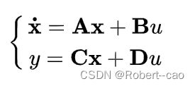
对于线性连续系统，状态空间方程为：

状态方程：

得：

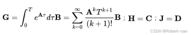
2. 零阶保持离散化

零阶保持法是在被离散对象前加零阶保持器，然后一起Z变换后离散化，已知一定常连续系统(SISO)的状态空间方程为：

 则对上式加入零阶保持器后Z变换得到:

 其中： T 为采样周期

 

 关于这个方程的推导可以看这篇博客：

线性连续时间状态空间模型的离散化及实例_Stan Fu的博客-CSDN博客_状态空间离散化

凸包:一系列点构成的凸包(V-representation)改为半空间的交集(H-representation)：

function [A_all, b_all]=obstHrep(nOb, vOb, lOb)

	% do simple checks
	if nOb ~= length(lOb)
		fprintf("ERROR in number of obstacles")
	end

	% these matrices contain the H-rep
	A_all = zeros(sum(vOb)-nOb,2)
	b_all = zeros(sum(vOb)-nOb,1)

	%counter for lazy people
	lazyCounter = 1;

	for i = 1 : nOb	% building H-rep
	
		A_i = zeros(vOb(i)-1,2);
		b_i = zeros(vOb(i)-1,1);
	
		% take two subsequent vertices, and compute hyperplane
		for j = 1 : vOb(i)-1

			% extract two vertices
			v1 = lOb(:,j);		%vertex 1
			v2 = lOb(:,j+1);	%vertex 2
		
			% find hyperplane passing through v1 and v2
			if v1(1) == v2(1)	% perpendicular hyperplane, not captured by general formula
				if v2(2) < v1(2)  % line goes "down"
					A_tmp = [1 0]
					b_tmp = v1(1)
				else
					A_tmp = [-1 0]
					b_tmp = -v1(1)
				end
			elseif v1(2) == v2(2) % horizontal hyperplane, captured by general formula but included for numerical stability
				if v1(1) < v2(1)
					A_tmp = [0 1]
					b_tmp = v1(2)
				else
					A_tmp = [0 -1]
					b_tmp = -v1(2)
				end
			else   % general formula for non-horizontal and non-vertical hyperplanes
				ab = [v1(1) 1 ; v2(1) 1] \ [v1(2) ; v2(2)]%y=k*x+b
				a = ab(1)
				b = ab(2)
			
				if v1(1) < v2(1)  %v1 --> v2 (line moves right)
					A_tmp = [-a 1]
					b_tmp = b
				else  % v2 <-- v1 (line moves left)
					A_tmp = [a -1]
					b_tmp = -b
				
				end
			end
			%# store vertices
			A_i(j,:) = A_tmp
			b_i(j) = b_tmp
		end
% 	
% 		# store everything
% 		A_all[lazyCounter : lazyCounter+vOb[i]-2,:] = A_i
% 		b_all[lazyCounter : lazyCounter+vOb[i]-2] = b_i
% 	
% 		# update counter
% 		lazyCounter = lazyCounter + vOb[i]-1
	end

	

end

Finding the Area of Irregular Polygons

1. Write down the coordinates of the vertices[3] of the irregular polygon. Determining the area for an irregular polygon can be found when you know the coordinates of the vertices.[4]

2. Create an array. List the x and y coordinates of each vertex of the polygon in counterclockwise order. Repeat the coordinates of the first point at the bottom of the list.

3. 

   3

   Multiply the x coordinate of each vertex by the y coordinate of the next vertex. Add the results. The added sum of these products is 82.

4. 4

   Multiply the y coordinate of each vertex by the x coordinate of the next vertex. Again, add these results. The added total of these products is -38.

5. 

   5

   Subtract the sum of the second products from the sum of the first products. Subtract -38 from 82 to get 82 - (-38) = 120.

6. 6

   Divide this difference by 2 to get the area of the polygon. Just divide 120 by 2 to get 60 and you're all done.

Matlab calculate the area of a polygon:

function s = CalculateArea(x, y)
% This function is used to calculate the area of a polygon.

x1 = x(1);
x2 = x(2);
x3 = x(3);
x4 = x(4);

y1 = y(1);
y2 = y(2);
y3 = y(3);
y4 = y(4);

s = 0.5 * abs(x1 * y2 + x2 * y3 + x3 * y1 - x1 * y3 - x2 * y1 - x3 * y2) + 0.5 * abs(x1 * y4 + x4 * y3 + x3 * y1 - x1 * y3 - x4 * y1 - x3 * y4);

Area of a polygon(Coordinate Geometry)

A method for finding the area of any polygon when the coordinates of its vertices are known.

(See also: Computer algorithm for finding the area of any polygon.)

First, number the vertices in order, going either clockwise or counter-clockwise, starting at any vertex.

 

The area is then given by the formula

 

Where xn is the x coordinate of vertex n,
yn is the y coordinate of the nth vertex etc.

The vertical bars mean you should make the reult positive even if it calculates out as negative.

Notice that the in the last term, the expression wraps around back to the first vertex again.

Try it here

Adjust the quadrilateral ABCD by dragging any vertex. The area is calculated using this method as you drag. A detailed explanation follows the diagram.

The above diagram shows how to do this manually.

1. Make a table with the x,y coordinates of each vertex. Start at any vertex and go around the polygon in either direction. Add the starting vertex again at the end. You should get a table that looks like the leftmost gray box in the figure above.
2. Combine the first two rows by:
   1. Multiplying the first row x by the second row y. (red)
   2. Multiplying the first row y by the second row x (blue)
   3. Subtract the second product form the first.
3. Repeat this for rows 2 and 3, then rows 3 and 4 and so on.
4. Add these results, make it positive if required, and divide by two.